Learning a foreign language is time-consuming.
If you were learning English as a foreign language, you would have a wealth of resources at your disposal. You would be using monolingual dictionaries built with a controlled vocabulary, not unlike Wikipedia's "simple English", i.e., the definitions would use a limited set of 2000 words, assumed to be known by the users, with exceptions dutifully highlighted. You would be provided with sample sentences, showing in which context and with which grammatical structure words should be used. You would also have lists of collocations -- collocations are pairs of words that often appear together: you can think of them as "minimal sample sentences".
For other languages, the learning materials are less adequate.
In this note, we will see how to automatically generate some of those missing resources, taking Japanese (and sometimes English) as an example.
First, we need a corpus, i.e., a set of texts, from which we can extract sample sentences, and which will tell us how often each word is used. We will use the Japanese wikipedia. It may sound unreasonable -- it is a 1GB file that uncompresses to more than 10GB -- but as long as the file remains compressed, this will not pose any problem.
# Check http://download.wikimedia.org/
# for more details and other languages.
# Take the pages-articles.xml file for "jawiki".
wget http://download.wikimedia.org/jawiki/20110921/jawiki-20110921-pages-articles.xml.bz2
ln -s jawiki-20110921-pages-articles.xml.bz2 jawiki-pages-articles.xml.bz2
We could also use newspaper articles, or novels in the public domain: from the Gutenberg project for western languages, from Aozora Bunko (青空文庫) for Japanese -- but for the latter, the spelling tends to be archaic (ゐる instead of いる, no small hiragana or katakana (しゃ,きゅ,はっ), etc.), the encoding is rarely specified, and the file formats are not always usable (text, HTML, but also PDF or GIF).
http://www.gutenberg.org/
http://www.aozora.gr.jp/
Wordnet is a list of English synonyms, with relations (antonymy, hyponymy etc.) between synonym sets.
This can be seen as an ontology. An ontology is a controlled vocabulary (for instance, there is one for human diseases, to make sure that everyone talks about the same thing when they use the same word), with relations between them (generalisation, specification, etc.), with all ambiguities removed -- therefore, strictly speaking, wordnet is not an ontology, since it explicitly describes polysemy.
# For more details: http://wordnet.princeton.edu
# Installation:
apt-get install wordnet
# Comman-line interface:
man wordnet
wn cat
wn cat -treen
wn cat -n1 -hypern
# Manually extract the synonym sets from the database:
perl -n -e '
  next if m/^\s/;  # Comments
  s/[|].*//;       # Glosses
  s/[0-9]//g;      # Remove all numbers
  s/\s\S\s/ /g;    # Remove all 1-character elements
  s/\s[^\sa-zA-Z][a-z]\s/ /g; # Also remove 2-character
                              # elements when the first
                              # is not a letter (%s, etc.)
  print
' /usr/share/wordnet/data.noun | head -100
Word dictionary:
# For more details, and more (specialized) dictionaries:
# http://ftp.monash.edu.au/pub/nihongo/00INDEX.html
# The old format is easier to use,
# but you may prefer the newer JMdict.gz (XML)
wget http://ftp.monash.edu.au/pub/nihongo/edict.gz
wget http://ftp.monash.edu.au/pub/nihongo/examples.gz
Kanji dictionary:
wget http://ftp.monash.edu.au/pub/nihongo/kanjidic.gz
wget http://ftp.monash.edu.au/pub/nihongo/kanjd212.gz
wget http://ftp.monash.edu.au/pub/nihongo/kradfile.gz
wget http://ftp.monash.edu.au/pub/nihongo/radkfile.gz
Convert those files to UTF8:
for i in edict kanjidic kanjd212 kradfile radkfile examples edict
do
  gzip -dc $i.gz | iconv -f EUC-JP -t UTF-8 | bzip2 -c > $i-utf8.bz2
done
We also need some description of the grammar of the language, at the very least, to help us identify words in a text.
For a language such as English, that would be relatively easy, since words are (usually) separated by spaces. However, we would have to be careful to "stem" (dis-inflect) the words, so that "car" and "cars" be recognised as the same word. We may also want to remove from the analysis extremely common words ("stop words") such as "a", "the", "and", etc.
Since, in Japanese, there are no spaces between words, it is trickier. It could be done as follows: take the list of all words in a dictionary, inflect them in all possible ways (you should have around one million strings), and look for those inflected forms in the text to analyze, with a preference for longer matches. If you store the inflected forms in a prefix tree, a greedy algorithm can do a reasonably good job -- you may want to add some backtracking for better results. However, there are more elaborate algorithms, based on the same idea (take all the words in a dictionary) but with a probabilistic twist (use a hidden Markov chain or a random grammar, for better results in case of ambiguity).
http://mecab.sourceforge.net/
There is a widespread confusion between character set and encoding. Many character sets have a single preferred encoding with the same name (ASCII, latin-1, etc.), but the Unicode character set has many encodings, and most character sets can be encoded using any of the Unicode encodings.
A character set is a set of characters, without any reference to the way they will be encoded; the characters are identified by a name (say "Latin letter A") or a number (just their rank in an ordered list) or both. Unicode is a character set.
An encoding is a way of encoding the characters in a character set, for instance, "write the rank of the character on two bytes" or "write the rank of the characters on two bytes and invert them" or "if the characters happens to be in the ASCII character set, use the ASCII encoding, otherwise, use two bytes, with their 8th bit set to 1, and code the rank of the character using the remaining 14 bits". UTF-8, UTF-16 (formerly UCS-2) and UTF-32 are the most common Unicode encodings.
We will mainly use Unicode and the UTF-8 encoding.
The designers of the Unicode character set tried to reduce the number of Asian characters as follows: when two different characters were very similar and had the same origin but were not used both in the same language, they were considered to be the same character.
That design decision is not unlike the omission, in the Latin1 character set, of the œ character, needed to write French (if you write this character as "oe", at school, it is considered a spelling mistake) -- but with thousands of characters.
As a consequence, there is no such thing as a complete "Unicode font": if it includes Asian characters, these will be either Chinese characters or Japanese characters, and cannot be used with with the other language, unless you are willing to scatter your text with spelling mistakes...
In other words, Unicode is not a character set for multilingual texts, but for monolingual texts -- it can be any language, but there has to be only one language. If you want several languages, you need something else (e.g., some XML markup) to separate and identify the languages.
The elements of the Unicode character set are not characters, but "code points": most are characters, but some are designed to be combined with another code point to form a single character. For instance, "combining tilde" (U+0303) is not a character by itself: it just indicates that there should be a tilde on the preceding character.
As a result, counting the number of characters in a string is not straightforward.
Some characters can be represented in several different ways in Unicode. For instance, this happens with accents: ñ (U+00F1) can also be represented as U+006E followed by U+0303 (Latin lower-case 'n' followed by the "combining tilde").
This makes checking for string equality, computing checksums, inserting strings in hash tables problematic.
This is a general-purpose encoding converter: we will use it to ensure that everything is in UTF-8.
To have the list of known encodings (the most important for us are UTF8; EUC-JP, SJIS, ISO-2022-JP; ISO-8859-1):
iconv -l
To convert from UTF8 to EUC-JP, discarding invalid characters (if the input file is corrupted) and inconvertible characters (they exist in the input character set but not in the output one):
iconv -c -f UTF8 -t EUC-JP
Even though Unicode should now be omnipresent, few, if any, programming languages use it transparently: it is not possible to tell the computer, once and for all, that "everything is in UTF8" and completely forget about it.
Perl can process UTF8 text, in the input files and the code (in particular, in the regular expressions), but you have to explicitly ask for it. The following seems to suffice (-CSDA is for the input and output, the utf8 module is for the strings and regular expressions that may appear in the code):
perl -CSDA -Mutf8
The -CSDA flags have to be on the command line, not on the first line of the file: Perl has to know it before the file is opened. In a script, you can use
#!perl -w
use utf8;
die "usage: perl -CSDA $0" unless ${^UNICODE} == 63;
Python's awareness of Unicode and UTF8 is rather recent. In Python 2, you have to explicitly specify the coding used in the source file and convert between strings of bytes and strings of Unicode characters; the "codecs" module automates part of the task (reading and writing UTF8 files).
#!/usr/bin/env python
# -*- coding: utf-8 -*-
unicode_string = unicode(utf8_string, errors='ignore')
unicode_string = utf8_string.decode('utf8', "ignore")
unicode_string = u'こんにちは'
utf8_string = unicode_string.encode('utf8') # In print() or write() statements
Things are slightly more transparent in Python 3: the source code is assumed to be in UTF8, all strings are in Unicode (no need for the u'...' syntax), it is no longer necessary to explicitly decode strings before printing them, and you can replace codec.open() with open().
In Java, char, Character and String are in Unicode and file read and writes will use the encoding specified by your default locale, unless you override it. Since the official documentation manages to confuse character set and encoding, character and code point, I would be very surprised if everything went smoothly...
Javascript is supposed to be more Unicode-aware than most "old" languages, but you still have to specify the encoding twice: in the header (if you inject UTF8 text in the document, the document had better be in UTF8) and the <script> blocks.
<meta http-equiv="Content-Type"; content="text/html; charset=utf-8"/>
<script type="text/javascript" src="[path]/myscript.js" charset="utf-8"></script>
In C or C++, you need a separate library to process Unicode, e.g., libiconv, GLib, ICU. The only standard things are the wchar_t and std::wstring types, for wide characters in general -- nothing Unicode-specific or Unicode-aware.
Unicode regular expressions are described here:
http://www.regular-expressions.info/unicode.html
Membership to a set of Unicode characters is represented as
\p{...}   Some property
\P{...}   The negation of that property
The following may be useful:
\p{Hiragana}
\p{Katakana}
\p{Han}                # Kanji
I sometimes use the following as well:
[^\x{2E80}-\x{F8FF}]   # Non-Asian characters
\P{Zs}                 # Space
\p{Ps} \p{Pe}          # Opening and closing brackets or quotes
Examples:
# Extract the Hiragana from a text, count them,
# and sort them from the most to the least frequent
cat sample-utf8.txt |
  perl -CSDA -Mutf8 -nle 'while(m/(\p{Hiragana})/g){print$1}' |
  sort | uniq -c | sort -nr

# Katakana
cat sample-utf8.txt |
  perl -CSDA -Mutf8 -nle 'while(m/(\p{Katakana})/g){print$1}' |
    sort | uniq -c | sort -nr

# Kanji
cat sample-utf8.txt |
  perl -CSDA -Mutf8 -nle 'while(m/(\p{Han})/g){print$1}' |
  sort | uniq -c | sort -nr
Since our aim is to produce learning materials (lists of words, sample sentences, dictionaries, etc.), we need some way of creating PDF files. OpenOffice is one solution.
You can use Perl to create an OpenOffice document in UTF8, from a template as follows (I use this to print vocabulary):
#! perl -w
use strict;
use utf8;
die "usage: perl -CSDA $0" unless ${^UNICODE} == 63;
use OpenOffice::OODoc;
ooLocalEncoding 'utf-8';  # To avoid the "Wide character in subroutine entry..." error message
use Encode;
# Template: an empty document,
# with the correct font, paper size, footer, styles.
my $document = odfDocument(file => '1.odt');
# The standard input (vocabulary list) should look like:
#   * Title
#   ~になぞらえる to liken to
#   君臨する(くんりん) to reign (dictator)
#   政権を掌握(しょうあく) seize (power)
while (my $line = <>) {
  my $style = ( $line =~ s/^\*\s*// ) ? "Heading" : "Default";
  print "LINE: $line";
  next if $line =~ m/^\s*$/;
  #if( m/^  ([^\s]+)  [(] ([^\s]+) [)] \s+ (.+) /x ) {
  #if( $line =~ m/^  (\P{Zs}+)  \p{Ps}  (\P{Zs}+) \p{Pe}  \p{Zs}* (.+) /x ) {
  if( $line =~ m/^
    (\P{Space_Separator}+)
    \p{Open_Punctuation}
    (\P{Space_Separator}+)
    \p{Close_Punctuation}
    \p{Space_Separator}*
    (.+)
  /x ) {
    $line = "$1\t$2\t$3";
    print "  SIMPLE: $1 | $2 | $3\n";
  #} elsif( $line =~ m/^ (\P{Zs}+) \p{Ps}+ (\P{Zs}+) /x ) {
  } elsif( $line =~ m/^
    (\P{Space_Separator}+)
    \p{Space_Separator}+
    (\P{Space_Separator}+)
  /x ) {
     $line = "$1\t\t$2";
    print "  NO PRONUNCIATION: $1 | | $2\n";
  } else {
    print "  Weird line\n";
  }
  $line = encode( 'utf8', $line );  # This is sometimes needed, sometimes not...
  $document->appendParagraph(
    text    => $line,
    style   => $style
  );
}
$document->save;
To produce PDF documents, I tend to use (La)TeX rather that its graphical competitors: it is much easier to automate.
Nowadays, (La)TeX documents are compiled with PdfTeX, XeTeX, or perhaps even luaTeX.
PdfTeX is almost identical to the traditional tex, but produces PDF files instead of DVI files. It is probably what you are using.
XeTeX also produces PDF files, but uses UTF8 by default and can transparently use any font (TrueType, Type1, OpenType) installed on your computer, even if it contains ligatures or variants -- you just need to know the name of the font. For instance, Japanese text can be typeset as:
{\fontspec{Sazanami Gothic}今日は}
LuaTeX is more recent, less mature, but should eventually replace PdfTeX. While TeX is a full-fledged programming language (some people write Basic or Lisp interpreters in TeX), it is very hard to use it as a programming language. This is not really due to the nature of the language, based on macro expansions (Metafont is based on the same idea and is perfectly usable), but to the fact that the text to be typeset is mixed with the code. A more familiar programming language (Python, etc.) and a better separation between code, markup and text would make LaTeX easier to use and extend. This is what LuaTeX is attempting to do. Lua, rather than Python, was chosen as the programming language -- it is widely used, as a scripting language, in the gaming industry, but almost unknown elsewhere.
Since our main corpus, Wikipedia, is in XML, we may need something to process XML files.
There are two types of APIs to process XML files.
DOM (Document Object Model)-type APIs represent the file as a tree, with each well-formed (i.e., with matching <> and </>) XML chunk forming a node, and you can move from node to node, by looking at the parent, children or siblings. To more easily access nodes or sets of nodes, there is often a regular-expression-like search API, for instance XPath.
In Perl, we could use the XML::LibXM module.
DOM is the most versatile and easy-to-use API, but it usually loads the whole document in memory: for large, database-like documents, it is not useable.
SAX-type APIs consider XML streams: start tag, end tag and text events form a stream, and the programmer can attach callback functions to each such event.
In Perl, you could use XML::SAX::Expat (and XML::SAX::Machines).
It is possible to combine the two approaches by cutting large files into chunks (e.g., Wikipedia into its articles) and processing each chunk in a DOM-like fashion (in Perl, one could use XML::Twig).
Finally, there is the quick-and-dirty way: just discard anything that looks like XML.
perl -p -e 's/<.*?>//g'
This is not entirely satisfactory (the < and > characters could appear inside quotes, the XML tags can span several lines, CDATA blocks are ignored, entities (<, etc.) are not expanded, etc.), but will suffice for our purposes.
Mecab allows you to cut Japanese sentences into words, to deconjugate verbs or adjective, and also gives you the pronunciation of the kanji as they appear in the text. (Prior to using mecab, I was using the Chasen morphological analyzer, but it was not reliable: it would often hang for no obvious reason and was therefore unusable on large texts such as Wikipedia.)
Here is a sample of the output produced.
$ cat test.utf8
猫は鼠を追っています。
$ cat test.utf8 | mecab
猫      名詞,一般,*,*,*,*,猫,ネコ,ネコ
は      助詞,係助詞,*,*,*,*,は,ハ,ワ
鼠      名詞,一般,*,*,*,*,鼠,ネズミ,ネズミ
を      助詞,格助詞,一般,*,*,*,を,ヲ,ヲ
追っ    動詞,自立,*,*,五段・ワ行促音便,連用タ接続,追う,オッ,オッ
て      助詞,接続助詞,*,*,*,*,て,テ,テ
い      動詞,非自立,*,*,一段,連用形,いる,イ,イ
ます    助動詞,*,*,*,特殊・マス,基本形,ます,マス,マス
。      記号,句点,*,*,*,*,。,。,。
EOS
It can be used to extract the words (in dictionary form) from a text:
cat test.utf8 | mecab |
  perl -CSDA -Mutf8 -n -l -e 'm/\t([^,]+,){6}([^,]+)/&&print$2'
# Or, equivalently:
cat sample-utf8.txt | mecab |
  perl -n -e 's/.*\t// && print' |
  cut -d, -f7
There is R package to access Mecab, but it can be tricky to install (it is not on CRAN) and not designed for large datasets: we will not use it.
http://rmecab.jp/wiki/index.php?RMeCab
In English we would only need to stem the words, e.g. with the Lingua::Stem module in Perl (there are also PoS-tagger in the Lingua::* namespace).
R also has a few NLP capabilities, but centered on English and not adequate for large corpuses: we will not use them.
http://cran.r-project.org/web/views/NaturalLanguageProcessing.html
All the characters and their number of occurrences:
bzip2 -dc jawiki-pages-articles.xml.bz2 |
  perl -CSDA -Mutf8 -p -e 's/(.)/$1\n/g' |
  perl -CSDA -Mutf8 -n -l -e '
    chomp;
    $a{$_}++;
    END{
      foreach(keys%a){
        print"$a{$_} $_"
      };
    }' |
  sort -n > characters
All the hiragana and their frequencies (the most frequent are のるに):
bzip2 -dc jawiki-pages-articles.xml.bz2 |
  perl -CSDA -Mutf8 -p -e '
    s/\P{Hiragana}//g;
    s/(.)/$1\n/g
  ' |
  perl -CSDA -Mutf8 -n -l -e '
    chomp;
    $a{$_}++;
    END{
      foreach(keys%a){
        print"$a{$_} $_"
      };
    }' |
  sort -n > hiragana
All the katakana and their frequency (the most frequent are ンスル):
bzip2 -dc jawiki-pages-articles.xml.bz2 |
  perl -CSDA -Mutf8 -p -e '
    s/\P{Katakana}//g;
    s/(.)/$1\n/g
  ' |
  perl -CSDA -Mutf8 -n -l -e '
    chomp;
    $a{$_}++;
    END{
      foreach(keys%a){
        print"$a{$_} $_"
      };
    }' |
  sort -n > katakana
All the kanji and their frequency (well, all the Asian characters except hiragana and katakana -- the punctuation is still there; the most common, in this file, are 年日月大本学人国中一市出作者部名会行用地道合場):
bzip2 -dc jawiki-pages-articles.xml.bz2 |
  perl -CSDA -Mutf8 -p -e '
    s/[^\x{2E80}-\x{F8FF}]//g; # Remove non-asian characters
    s/\p{Hiragana}//g;         # Remove hiragana
    s/\p{Katakana}//g;         # Remove katakana
    s/(.)/$1\n/g
  ' | perl -CSDA -Mutf8 -n -l -e '
    chomp;
    $a{$_}++;
    END{
      foreach(keys%a){
        print"$a{$_} $_"
      };
    }' |
  sort -n > kanji
An N-gram is just a sequence of N characters in a text. For instance, you can easily recognize the language of a text by looking at the 1-grams (i.e., the letter frequencies) or, better, the 2-grams it contains.
Let us look at the N-gram frequencies of texts in various (Western) languages languages (retrieved from the GUTenberg project).
# A. C. Doyle
http://www.gutenberg.org/dirs/etext99/advsh12.zip
http://www.gutenberg.org/files/2097/2097.zip
http://www.gutenberg.org/files/108/108.zip
http://www.gutenberg.org/files/834/834.zip
http://www.gutenberg.org/files/2852/2852.zip

# M. Twain
http://www.gutenberg.org/files/76/76.zip
http://www.gutenberg.org/files/74/74.zip
http://www.gutenberg.org/files/119/119.zip

# L. Caroll
http://www.gutenberg.org/files/11/11.zip
http://www.gutenberg.org/files/13/13.zip
http://www.gutenberg.org/dirs/etext96/sbrun10.zip
http://www.gutenberg.org/files/12/12.zip

# J. Verne
http://www.gutenberg.org/dirs/etext04/820kc10.txt
http://www.gutenberg.org/dirs/etext03/7vcen10.zip
http://www.gutenberg.org/dirs/etext97/780jr07.zip
http://www.gutenberg.org/dirs/etext04/8robu10.txt
http://www.gutenberg.org/files/14287/14287-8.zip
After downloading and uncompressing those files, we can count the 2-grams in each.
for i in *txt
do
  cat $i | perl -n -l -e '
    y/A-Z/a-z/;
    s/[^a-z]//g;
    for($i=0;$i<=length($_)-2;$i++){
      $a{ substr($_,$i,2) }++
    }
    END{
      foreach $k (keys %a) {
        print "$k,$a{$k}";
      }
    }
  ' |
  perl -p -e "s/^/$i,/"
done > a.csv
In R:
library(reshape2)
d <- read.csv("a.csv",header=FALSE)
names(d) <- c("file","ngram","number")
d$file <- gsub("\\.txt$", "", as.character(d$file))
x <- dcast(d, file ~ ngram, value="number")
rownames(x) <- as.character(x$file)
x <- x[,-1]
x[ is.na(x) ] <- 0
x <- x / apply(x,1,sum)
stopifnot( apply(x,1,sum) == 1 )
plot(hclust(dist(x)))
doyle  <- c("advsh12","2097","108","834","2852")
twain  <- c("76","74","119")
caroll <- c("11","12","13","sbrun10")
verne <- c("820kc10","7vcen10","780jr07","8robu10","14287-8")
authors <- rbind(
  data.frame(author="A.C.Doyle",file=doyle),
  data.frame(author="M.Twain",  file=twain),
  data.frame(author="L.Caroll", file=caroll),
  data.frame(author="J.Verne",  file=verne)
)
authors$file <- paste(authors$file, "txt", sep=".")
authors$author <- as.character(authors$author)
rownames(authors) <- as.character(authors$file)
authors[rownames(x),"author"]

y <- cmdscale(dist(x),2)
plot(y, type="n", xlab="", ylab="", main="2-grams and language identification", axes=FALSE)
box()
text(y, authors[rownames(y),"author"] )
Identifying the author is not straightforward -- we would probably need to clean the files more carefully (the licence is still there...) and look at word usage.
i <- which(authors[rownames(x),"author"] != "J.Verne")
y <- cmdscale(dist(x[i,1:20]),2)
plot(y, type="n", xlab="", ylab="", main="2-grams and author identification", axes=FALSE)
box()
text(y, authors[rownames(y),"author"] )
In Japanese,
bzip2 -dc jawiki-pages-articles.xml.bz2 |
  perl -n -l -CSDA -Mutf8 -e '
    s/[^\p{Han}\p{Hiragana}\p{Katakana}]//g;
    for($i=0;$i<=length($_)-2;$i++)
    { $a{ substr($_,$i,2) }++ }
    END{ foreach $k (keys %a) { print "$a{$k},$k" } }
  ' | sort -rn > 2grams
bzip2 -dc jawiki-pages-articles.xml.bz2 |
  mecab |
  perl -CSDA -Mutf8 -n -l -e 'm/\t([^,]+,){6}([^,*]+)/ && print$2' |
  perl -CSDA -Mutf8 -n -l -e 'chomp;$a{$_}++;END{foreach(keys%a){print"$a{$_} $_"};}' |
  sort -rn > words
Since this will be useful later, let us store this data is a more directly usable format.
perl -CSDA -Mutf8 -MStorable -n -e '
  $a{$2} = $1 if m/^(.+?)\s+(.+?)\s*$/;
  END{ store \%a, "words.bin" }
' words
bzip2 -dc jawiki-pages-articles.xml.bz2 |
  perl -CSDA -Mutf8 -n -l -e '
    m#<title>(.*)</title># && {$jp=$1};
    m/^\[\[en:(.*)\]\]/ && {print "$jp\t$1"}
  ' > translations_from_wikipedia
(The problem is taken from a quiz.)
All 2-character words:
gzip -dc edict.gz | iconv -f EUC-JP -t UTF8 |
  perl -CSDA -Mutf8 -n -l -e 'm/^(..) / && print $1'
All 2-character words containing those characters:
gzip -dc edict.gz | iconv -f EUC-JP -t UTF8 |
  perl -CSDA -Mutf8 -n -l -e 'm/^([分似人親].|.[分似人親])/ && print $1'
The solution:
characters="分似人親"
gzip -dc edict.gz | iconv -f EUC-JP -t UTF8 |
  perl -CSDA -Mutf8 -n -l -e 'm/^((['"$characters"'])(.)|(.)(['"$characters"']))/ && print "$3$2$4$5"' |
  sort | uniq |
  perl -CSDA -Mutf8 -p -e 's/^(.)./$1/' |
  uniq -c | grep 4
Word usage changes with time, and this can reveal changes on how we view the world. For instance, some claim that as economic bubbles grow, newspapers tend to use the word "new" (or synonyms, such as "2.0") more often.
http://books.google.com/ngrams/graph?content=new%2Cold&year_start=1980&year_end=2012&corpus=0&smoothing=0
The same analysis can be generalized to the blogs or microblogs (twitter), to whole semantic categories instead of isolated words (replace "new" by all the words expressing novelty, or all positive words, or all negative words, etc.), specialized to texts containing a certain word (e.g., the name of a company in which you may want to invest), etc.
http://arxiv.org/abs/1101.5120
http://arxiv.org/abs/1010.3003
http://www.rinfinance.com/agenda/2011/JoeRothermich.pdf
(The lists of words used by those articles do not seem to be freely available.)
mecab | perl -ne 'print if s/.*\t//' | cut -d, -f1 |
perl -n -e '
  print "$previous -> $_" if $previous;
  chomp();
  $previous = $_
' |
sort | uniq -c | sort -nr | head -n 10 |
perl -p -e '
  BEGIN{print"digraph G {\n";}
  chomp;
  s/^\s*([0-9]+)\s+(.*)/  $2 [label="$1"];\n/;
  END{print"}\n";}
' > result.dot
# Use GraphViz to plot the graph: http://www.graphviz.org/
dot -Tsvg result.dot > result.svg
The plot would be more readable with probabilities, in percent, rather than number of occurrences.
bzip2 -dc jawiki-pages-articles.xml.bz2
mecab | perl -ne 'print if s/.*\t//' | cut -d, -f1 |
perl -n -e '
  print "$previous $_" if $previous;
  chomp();
  $previous = $_
' |
sort | uniq -c | sort -nr | perl -p -e 's/^\s*//' > tmp.csv
echo '
d <- read.csv("tmp.csv",sep=" ",header=FALSE)
library(reshape2)
d <- dcast(d, V2~V3,value.var="V1")
rownames(d) <- as.character(d[,1])
d <- as.matrix(d[,-1])
d[ is.na(d) ] <- 0
# Transition probabilities, rounded, in percents
d <- round( 100 * d / apply(d,1,sum) )
# Reduce the number of nodes, to make the graph more readable
pos <- c(
  "名詞",   # Noun
  "助詞",   # Particle (like a preposition,
           # but it comes after the noun, not before --
           # declensions, in indo-european languages,
           # may once have been postpositions).
  "動詞",   # Verb
  "助動詞", # Verb inflection
  "形容詞", # Adjective
  "副詞",   # Adverb
  "記号"   # Symbol (punctuation)
)
d <- d[pos,pos]
# Remove small probabilities
cat("digraph G {\n")
for(i in 1:dim(d)[1]) {
  for(j in 1:dim(d)[2]) {
    if( d[i,j] > 20 ) {
      cat(rownames(d)[i], " -> ", colnames(d)[j])
      cat(" [label=\"", d[i,j], "%\"];\n", sep="")
    }
  }
}
cat("}\n")
' | R --vanilla --slave > result.dot
dot -Tsvg result.dot > result.svg
display result.svg

The results are somewhat biased: some of the grammatically important transitions have disappeared when we truncated the graph. For instance 名詞→助詞 is missing, even though nouns are almost always followed by a particle. What happens is that nouns can be concatenated, so that the noun→noun transitions outnumber the noun→particle transitions...
character=魔
gzip -dc edict.gz | iconv -f EUC-JP -t UTF8 |
  perl -CSDA -Mutf8 -n -e 'print if m#^[^/\[]*'"$character"'#'
There are too many results: we want the most common words among those. Let us use the word frequencies we stored earlier.
character=魔
gzip -dc edict.gz | iconv -f EUC-JP -t UTF8 |
  perl -CSDA -Mutf8 -MStorable -n -e '
    BEGIN{ %a = %{retrieve "words.bin"}; }
    next unless m#^([^/\[\s]*'"$character"'[^/\[\s]*)#;
    print $a{$1} // 0; print " $_";
  ' | sort -n
We can just grep in the example file:
bzip2 -dc examples-utf8.bz2 | perl -CSDA -Mutf8 -n -e '
  # Lines are grouped by pairs:
  # the first one starts with "A: "
  # and contains the sentence and a translation;
  # the second, starting with "B: ",
  # contains the words.
  if(m/^A:\s+(\S+)\s+(.+)\#/){ $sentence=$1; $translation=$2; }
  if(s/^B:\s+//){
    # Discard everything but the words in dictionary forms
    s/\(.*?\)//g; s/\{.*?\}//g; s/\[.*\]//g;
    @words=split(/\s+/);
    print "|" . join("|",@words) .
          "|   $sentence --> $translation\n"
  }' | fgrep '|整理|'
One problem with sample sentences, especially when they are extracted automatically, is that they can contain words much more complicated than the word you are interested in: we need some way of gauging the level of difficulty of each sentence. For instance, we can use the frequency of the rarest word it contains (after removing the word we are interested in).
word="整理"
bzip2 -dc examples-utf8.bz2 | perl -CSDA -Mutf8 -n -e '
  if(m/^A:\s+(\S+)\s+(.+)\#/){ $sentence=$1; $translation=$2; }
  if(s/^B:\s+//){
    s/\(.*?\)//g; s/\{.*?\}//g; s/\[.*\]//g;
    @words=split(/\s+/);
    print "|" . join("|",@words) .
          "|   $sentence --> $translation\n"
  }' |
  fgrep "|$word|" |
  perl -CSDA -Mutf8 -MStorable -MList::Util=max,min -n -e '
    BEGIN{ %a = %{retrieve "words.bin"}; }
    $line = $_;
    next unless s/\|'"$word"'\|/\|/;
    m/\|(.*)\|\s*(.*)/;
    $level = min( map {$a{$_} or 1e100} split("|",$1) );
    print "$level $2\n";
  ' | sort -n
We can do the same thing with a larger corpus: we just have to extract sentences and split them into words.
bzip2 -dc jawiki-pages-articles.xml.bz2 |
# Consider that line that ends with a 。 is a sentence.
perl -CSDA -Mutf8 -p -e 's/。/。\n/g' | fgrep 。 |
mecab |
perl -n -Mutf8 -CSDA -e '
  if( m/^EO/ && @words ) {
    print "|", join("|", @words), "| ", $sentence, "\n";
    @words = ();
    $sentence = "";
  } elsif( m/^(.*?)\t([^,]+),([^,]+),([^,]+),([^,]+),([^,]+),([^,]+),([^,]+),([^,]+)/ ) {
    push @words, "$8" if $2 ne "記号";
    $sentence .= $1;
  }
' | # We may want to store the processed sentences somewhere
fgrep "|$word|" |
perl -CSDA -Mutf8 -MStorable -MList::Util=max,min -n -e '
  BEGIN{ %a = %{retrieve "words.bin"}; }
  $line = $_;
  next unless s/\|'"$word"'\|/\|/;
  m/\|(.*)\|\s*(.*)/;
  $level = min( map {$a{$_} or 1e100} split("|",$1) );
  print "$level $2\n";
' | sort -n
We can do exactly the same thing in English -- the only difference is that we stem the words.
Extract sentences:
cat english_corpus.txt |
perl -p -e 's/[.]\s+/.\n/g' |
perl -p -e '
  next if m/^\s*$/;
  if( ! m/[.]\s*$/ ) {
    chomp;
    $_+=" ";
  }' |
perl -n -e 'print if m/^\s*[A-Z].*[.]/' > english_sentences.txt
Extract words from sentences:
cat english_sentences.txt |
perl -n -e '
  @words=split(/[^a-zA-Z]+/);
  print "[", join("][", @words), "]", $_
'
We also need to stem them:
cat english_sentences.txt |
perl -M'Lingua::Stem qw(stem)' -n -e '
  @words=split(/[^a-zA-Z]+/);
  $stemmed_words=stem(@words);
  print "[", join("][", @$stemmed_words), "]", $_
' > english_sentences_tagged.txt
Add a "difficulty level" to each sentence, depending on how rare the words it uses are.
cat english_sentences_tagged.txt |
perl -p -e 's/\]/\]\n/g;' |
perl -MStorable -n -e '
  chomp;
  $a{$_}++ if m/\[/;
  END{
    for $w (keys %a) {
      print $a{$w}, " ", $w, "\n"
    }
    store \%a, "english_words.bin";
  }' | sort -rn > english_words.txt
cat english_sentences_tagged.txt |
perl -MStorable -n -e '
  BEGIN{
    %a = %{retrieve "english_words.bin"};
  }
  $sentence = $_;
  s/\]/\]\|/g;
  @words = split(/\|/);
  @occurrences = map {$a{$_}} @words;
  @occurrences = sort @occurrences;
  print join(" ",@occurrences), " ", $sentence;
' > english_sentences_tagged_and_ranked.txt
It can be used as follows:
grep justice english_sentences_tagged_and_ranked.txt |
sort -rn |
perl -p -e 's/.*\]//'
Similar ideas could be applied to music: the Humdrum project (no update since 2005) was trying to do just that.
http://musicog.ohio-state.edu/Humdrum/
http://humdrum.ccarh.org/
Some pairs of words tend to be used together: for instance, うっそうと is often followed by した or 茂る (it is so systematic that could be seen as a fixed expression); 多様 is often used with 生み出す (this time, it is not a fixed expression). These are called collocations.
Since we will be dealing with pairs of words, the volume of data will be huge, and the Perl one-liner (i.e., disposable code) approach we have taken so far, completely disregarding performance issues, will no longer work.
The algorithm will be following:
1. Extract sentences from the corpus
2. Tag the sentences, i.e., identify the words
3. Count the number of sentences,
   the number of occurrences of each word
4. Count the number of occurrences of pairs of words
5. For each pair of words, compute the some "collocation score"
The tricky part is dealing with the pairs of words, because there are too many of them to fit in memory.
I tried the following approaches, but they did not work. Put the pairs of words in a hash table, in Perl, in memory -- this requires too much memory. Put the pairs of words in a hash table, in Perl, but when the table contains 1,000,000 elements, write it to disk (with the Storable module), merging it with the previous one -- the merging step was problematic. Put the pairs of words in a SQLite database, updating 1,000,000 pairs at a time -- the merging step was still problematic. Idem with MonetDB instead of SQLite -- same problem. Put the pairs in a 2-dimensional array, in C, to try to gain a better control on memory usage -- this was using too much memory.
A "divide-and-conquer" (now known as "map-reduce") approach proved more successful: put the pairs of words in a hash table, write it to disk when it reaches 1,000,000 elements, but write it in 256 different files.
Let us do it.
Extracting the sentences is straightforward if we allow some inaccuracies: let us consider that anything that ends with a period is a sentence.
bzip2 -dc jawiki-pages-articles.xml.bz2 |
grep '。$' | perl -p -Mutf8 -CSDA -e 's/。/。\n/g' |
bzip2 -c > sentences.bz2
To tag the sentences, just call mecab to extract the words and their PoS (part of speech); for future reference, we also keep the raw sentence.
# Example:
#   猫が鼠を食べた。
# becomes
#   (名詞,猫;助詞,が;名詞,鼠;助詞,を;動詞,食べる;助動詞,た)猫が鼠を食べた。
bzip2 -dc sentences.bz2 |
mecab |
perl -n -Mutf8 -CSDA -e '
  if( m/^EO/ && @words ) {
    print "(", join(";", @words), ")", $sentence, "\n";
    @words = ();
    $sentence = "";
  } elsif( m/^(.*?)\t([^,]+),([^,]+),([^,]+),([^,]+),([^,]+),([^,]+),([^,]+),([^,]+)/ ) {
    push @words, "$2,$8" if $2 ne "記号";
    $sentence .= $1;
  }
' |
bzip2 -c > tagged_sentences.bz2
We actually need slightly more than that: we also want pairs of words. The following extracts noun-particle-verb triplets.
bzip2 -dc tagged_sentences.bz2 |
perl -Mutf8 -CSDA -n -e '
  m/^\((.*?)\)(.*)$/;
  $words = $1;
  $sentence = $2;
  #print STDERR "SENTENCE: $sentence\n";
  @F = split(/;/, $1);
  #print STDERR "F: (", join("; ", @F), ")\n";
  @F = map { [ split(/,/,$_) ]} @F;
  #print STDERR "F[i]->[0]: (", join("; ", map {$_->[0]} @F), ")\n";
  #print STDERR "F[i]->[1]: (", join("; ", map {$_->[1]} @F), ")\n";
  @result = ();
  for($i=0; $i<=$#F; $i++) {
    #print STDERR "  POS: $F[$i][0]\n";
    next if $F[$i][0] ne "名詞";
    #print STDERR "  Noun: $F[$i][1]\n";
    $j=$i+1; # The particle should be immediately after the noun
    next unless $F[$j][0] eq "助詞";
    #print STDERR "    Particle: $F[$j][1]\n";
    for($k=$j+1; $k<=$#F; $k++) {
      if( $F[$k][0] eq "動詞" ) {
        push @result, "$F[$i][1]$F[$j][1],$F[$k][1]";
        last;
      }
    }
  }
  print "($words)", "(", join(";",@result), ")", $sentence, "\n";
  ' | bzip2 -c > fully_tagged_sentences.bz2
Let us count the sentences and the words. The results will be stored in a SQLite file.
bzip2 -dc fully_tagged_sentences.bz2 |
perl -MDBI -Mutf8 -CSDA -n -e '
  next unless m/^\(.*?\)\((.*?)\)/;
  @pairs = split(/;/,$1); # The collocation candidates
  my %a = ();
  my %b = ();
  foreach my $pair (@pairs) {
    @pair = split(",",$pair);
    $a{$pair[0]} = 1;
    $b{$pair[1]} = 1;
  }
  foreach my $word (keys %a) { $left{$word}++; }
  foreach my $word (keys %b) { $right{$word}++; }
  $sentences++;
  END{
    my $dbh = DBI->connect(
      "dbi:SQLite:dbname=collocations.sqlite",
      "","",{AutoCommit=>0}
    );
    $dbh->do("DROP TABLE IF EXISTS T0");
    $dbh->do("CREATE TABLE T0 (n DOUBLE)");
    my $sth = $dbh->prepare("INSERT INTO T0 (n) VALUES (?)");
    $sth->execute( $sentences );
    $dbh->commit;
    $dbh->do("DROP TABLE IF EXISTS T1");
    $dbh->do("CREATE TABLE T1 (k1 VARCHAR PRIMARY KEY, n1 INTEGER)");
    my $sth = $dbh->prepare("INSERT INTO T1 (k1,n1) VALUES (?,?)");
    foreach my $word (keys %left)
    { $sth->execute($word, $left{$word}); }
    $dbh->commit;
    $dbh->do("DROP TABLE IF EXISTS T2");
    $dbh->do("CREATE TABLE T2 (k2 VARCHAR PRIMARY KEY, n2 INTEGER)");
    my $sth = $dbh->prepare("INSERT INTO T2 (k2,n2) VALUES (?,?)");
    foreach my $word (keys %right)
    { $sth->execute($word, $right{$word}); }
    $dbh->commit;
    print "Sentences: $sentences\n";
    print "Left: ",  scalar keys %left,  "\n";
    print "Right: ", scalar keys %right, "\n";
  }
'
Now comes the tricky bit: counting word pairs. We periodically update the data on disk, splitting it into 256 buckets, determined by the first byte of the MD5 checksum.
bzip2 -dc fully_tagged_sentences.bz2 |
perl -Mutf8 -CSDA -MStorable -MDigest::MD5 -n -e '
  BEGIN {
    # MD5 does not like UTF8
    # (The UTF8 representation of a Unicode string
    # is not unique.)
    use Encode qw(encode_utf8);
  }
  sub f (\%) {
    my $a = shift;
    my $new_elements = scalar (keys %$a);
    print STDERR "Spitting those $new_elements elements\n";
    my %b;
    foreach $w (keys %$a) {
      my $y = substr(Digest::MD5::md5_hex(encode_utf8($w)), 0, 2);
      $b{$y} = {} unless exists $b{$y};
      $b{$y}->{$w} = $a->{$w};
    }
    print STDERR "Writing \n";
    $new_elements = 0;
    my $old_elements = 0;
    foreach my $y (keys %b) {
      print STDERR "$y ";
      my $old = $b{$y};
      if( -f "jawiki_words_$y.bin" ) {
        $old = retrieve "jawiki_words_$y.bin";
        $old_elements += scalar keys %$old;
        foreach my $w (keys %{ $b{$y} }) {
          $old->{$w} += $b{$y}->{$w};
        }
      }
      $new_elements += scalar (keys %$old);
      store $old, "jawiki_words_$y.bin";
    }
    %$a = ();
    print STDERR "\nNumber of elements: $old_elements --> $new_elements\n";
    print STDERR "Continuing\n";
  }
  m/\(.*?\)\((.*?)\)/;
  @w = split(/;/,$1);
  foreach $w (@w) { $a{$w}++ };
  f %a if scalar keys %a > 1_000_000;
  END { f %a; }
'
Aggregate, into a SQLite table:
perl -MDBI -MStorable -Mutf8 -CSDA -e '
  print STDERR "Connect\n";
  my $dbh = DBI->connect(
    "dbi:SQLite:dbname=collocations.sqlite",
    "","",{AutoCommit=>0}
  );
  print STDERR "Drop\n";
  $dbh->do("DROP TABLE IF EXISTS pairs");
  print STDERR "Create Table\n";
  #$dbh->do("CREATE TABLE pairs (k1 VARCHAR, k2 VARCHAR, n12 INTEGER, bucket INTEGER, PRIMARY KEY (k1, k2))");
  $dbh->do("CREATE TABLE pairs (k1 VARCHAR, k2 VARCHAR, n12 INTEGER, bucket INTEGER)"); # No primary key
  $dbh->commit();
  print STDERR "Committed\n";
  my $sth = $dbh->prepare("INSERT INTO pairs (k1,k2,n12,bucket) VALUES (?,?,?,?)");
  die unless $sth;

  for(my $i=0; $i<256; $i++) {
    my $y = sprintf("%x", $i);
    if( -f "jawiki_words_$y.bin" ) {
      print STDERR "$y ";
      my $a = retrieve "jawiki_words_$y.bin";
      foreach my $w (keys %$a) {
        my ($k1, $k2) = split(",",$w);
        #print STDERR "INSERT $k1, $k2\n";
        $sth->execute($k1, $k2, $a->{$w}, $i)
        if $a->{$w} > 1; # Discard pairs that only appear once
      }
      $dbh->commit(); # Only do this at the end?
    }
  }
  $dbh->commit();
  $dbh->disconnect();
  print STDERR "\n";
'
We can now compute a "score" to identify collocations. Several are commonly used.
http://pioneer.chula.ac.th/~awirote/colloc/statmethod1.htm
Mutual information and Pearson's chi squared are symmetric and biased towards rare words.
Mutual Information = p12 / ( p1 * p2 )
Chi Squared = Sum (Observed - Expected)^2 / Expected
            = ...
            = N * (p12 - p1 * p2 )^2 / ( p1 * p2 * (1-p1) * (1-p2) )
where
  p1  =  N1/N
  p2  =  N2/N
  p12 = N12/N
Dunning's log-likelihood may be preferable.
Dunning's log-likelihood =
  ( p^N2 * (1-p)^(N-N2) ) /
  ( p1^N12 * (1-p1)^(N1-N12) * p2^(N2-N12) * (1-p2)^(N-N1-N2+N12)
where
  p  = P(Word2|Word1) = P(Word2|¬Word1) (null hypothesis)
  p1 = P(Word2|Word1)
  p2 = P(Word2|¬Word1)
are estimated as
  p  = N2 / N
  p1 = N12 / N1
  p2 = N12 / N2
Mutual information and Chi squared can be computed directly in SQL.
echo '
  CREATE TABLE tmp AS
  SELECT *,
    p12/p1/p2 AS "Mutual Information",
    n * (p12 - p1*p2)*(p12 - p1*p2) / ( p1 * p2 * (1-p1) * (1-p2) ) AS "Chi2"
  FROM (
  SELECT
    pairs.k1, pairs.k2, n12, n1, n2, n, bucket,
    n1/n AS p1, n2/n AS p2, n12/n AS p12
  FROM pairs, T1, T2, T0
  WHERE pairs.k1 = T1.k1 AND pairs.k2 = T2.k2
  ) A;
  -- ORDER BY Chi2 DESC;
' | sqlite3 collocations.sqlite
We now need to add the log-likelihood. We could load the data into R (not the whole data, it is too large: one bucket at a time -- that is why I have kept the "bucket" column), add the log-likelihood column, and save the data back to SQLite. We could also use the SQLite::More Perl module, that adds, among other things, a logarithm function to SQLite.
Since the log-likelihood is not symmetric, we will want both variants: let us define a function to compute it -- SQLite allows us to define our own functions.
perl -MDBI -e '
  my $dbh = DBI->connect(
    "dbi:SQLite:dbname=collocations.sqlite",
    "","",{AutoCommit=>1}
  );
  print STDERR "Drop\n";
  $dbh->do("DROP TABLE IF EXISTS collocations");
  print STDERR "Create Function\n";
  $dbh->sqlite_create_function("dunning", 4, sub {
    my ($n,$n1,$n2,$n12) = @_;
    return undef if $n1<=0 or $n1<=0 or $n-$n1 <=0;
    my $p  = 1.0 * $n2  / $n;           # P[word 2]
    my $p1 = 1.0 * $n12 / $n1;          # P[word 2|word 1]
    my $p2 = 1.0 * ($n2-$n12)/($n-$n1); # P[word 2|not word 1]
    return undef if  $p*(1-$p)  <= 0;
    return undef if $p1*(1-$p1) <= 0;
    return undef if $p2*(1-$p2) <= 0;
    my $result =
      $n2 * log($p) + ($n-$n2)*log(1-$p)
      - $n12 * log($p1) + ($n1-$n12)*log(1-$p1)
      - ($n2-$n12) * log($p2) + ($n-$n1-$n2+$n12)*log(1-$p2);
    return $result;
  } );
  print STDERR "Create Table\n";
  $dbh->do( <<"EOQ" );
    CREATE TABLE collocations AS
    SELECT
        k1, k2, n12, n1, n2, n,
        CAST( "Mutual Information" AS DOUBLE ) AS MutualInformation,
        CAST( Chi2 AS DOUBLE ) AS Chi2,
        CAST( dunning(n,n1,n2,n12) AS DOUBLE) AS loglikelihood2,
        CAST( dunning(n,n2,n1,n12) AS DOUBLE) AS loglikelihood1
    FROM tmp;
EOQ
'
It seems to work, but the various metrics are not consistent...
SELECT *
FROM collocations
WHERE k1 = '必要が'
ORDER BY loglikelihood1
LIMIT 5; -- Much faster without "LIMIT"...
Store the results in a CSV file, for later use.
echo '
  .headers ON
  SELECT * FROM collocations LIMIT 5;
' | sqlite3 collocations.sqlite |
bzip2 -c > collocations.csv.bz2
Finally, clean the directory (4GB to delete):
rm -f jawiki_words_??.bin
rm -f sentences.bz2
rm -f tagged_sentences.bz2
rm -f fully_tagged_sentences.bz2
echo '
  DROP TABLE IF EXISTS tmp;
  DROP TABLE IF EXISTS pairs;
  DROP TABLE IF EXISTS T0;
  DROP TABLE IF EXISTS T1;
  DROP TABLE IF EXISTS T2;
' | sqlite3 collocations.sqlite
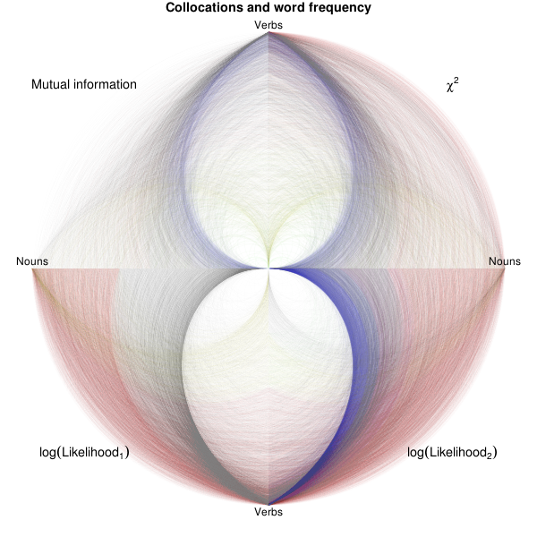
A hiveplot is just a parallel plot in polar coordinates, using transparency to accommodate a large number of observations. They are sometimes used to plot (graph-theoretic) graphs, especially if the usual graph layout algorithms do not provide any insight on the structure of the graph.
http://www.hiveplot.org/
http://www.hiveplot.org/talks/linnet-introduction.pdf
http://www.hiveplot.org/talks/hive-plot.pdf
In the plot at the beginning of this note, verbs and nouns are on separate axes. The farther away from the origin, the more frequent the words are. The opacity in each quadrant is determined by the various metrics used to identify collocations.
library(sqldf)
d <- read.csv("collocations.csv.bz2", sep="|", nrows=1e4)
d <- d[apply(d, 1, function(x) !any(is.na(x))),]
nouns <- d[!duplicated(d$k1),c("k1","n1")]
nouns$position1 <-
  rank( nouns$n1, ties.method = "random" ) / length(nouns$n1)
verbs <- d[!duplicated(d$k2),c("k2","n2")]
verbs$position2 <-
  rank( verbs$n2, ties.method = "random" ) / length(verbs$n2)
d <- sqldf("
  SELECT d.k1, d.k2, nouns.position1, verbs.position2,
         MutualInformation, Chi2,
         loglikelihood2, loglikelihood1
  FROM d
  LEFT JOIN nouns ON d.k1 = nouns.k1
  LEFT JOIN verbs ON d.k2 = verbs.k2;
")
# Make sure all the measures are in [0,1]
d$loglikelihood1 <- log(-d$loglikelihood1)/255
d$loglikelihood2 <- log(-d$loglikelihood2)/255
d$MutualInformation <- 3*log(d$MutualInformation)/255
d$Chi2 <- 3*pmax(0,log(d$Chi2))/255
measures <- list(
  Chi2 = expression(chi^2),
  loglikelihood1 = expression(log(Likelihood[1])),
  loglikelihood2 = expression(log(Likelihood[2])),
  MutualInformation = "Mutual information"
)
# Convert (x,y) in [0,1]^2 into a colour,
# with red, green, blue, yellow in the corners.
f <- function(x,y,alpha=1) {
  w00 <- 1 /( 1e-6 + x+y )
  w10 <- 1 /( 1e-6 + (1-x)+y )
  w01 <- 1 /( 1e-6 + x+(1-y) )
  w11 <- 1 /( 1e-6 + (1-x)+(1-y) )
  c00 <- c(0,1,0)
  c10 <- c(1,1,0)
  c01 <- c(0,0,1)
  c11 <- c(1,0,0)
  colour <- ( w00*c00 + w10*c10 + w01*c01 + w11*c11 ) /
    (w00+w01+w10+w11)
  rgb(colour[1], colour[2], colour[3], alpha)
}
#f <- function(x,y,alpha=1) rgb(0,0,0,alpha)
#n <- 1000; x <- runif(n); y <- runif(n);
#plot(x,y,type="n");
#for(i in 1:n)
#{ points(x[i],y[i],pch=16,cex=2,col=f(x[i],y[i])) }
op <- par(mar=c(1,1,1,1))
plot(NA,
  xlim=c(-1,1), ylim=c(-1,1),
  axes=FALSE, xlab="", ylab="")
for(j in 1:4) {
  m <- c(
    "Chi2", "MutualInformation",
    "loglikelihood1", "loglikelihood2"
  )[j]
  theta1 <-  pi * ( j %% 3 - 1 )
  theta2 <- pi/2-pi*floor((j-1)/2)
  k <- 100
  theta <- seq(theta1, theta2, length=k)
  lambda <- seq(0,1, length=k)
  for(i in 1:dim(d)[1]) {
    r <- (1-lambda) * d$position1[i] + lambda * d$position2[i]
    alpha <- pmax(0,pmin( d[i,m] / dim(d)[1]*2e3, 1 ))
    lines(r*cos(theta), r*sin(theta),
      col=f(d$position1[i],d$position2[i],alpha))
  }
  text(
    1.1*cos((theta1+theta2)/2),1.1*sin((theta1+theta2)/2),
    measures[[m]],
    cex=1.2
  )
  #zeroes <- rep(0,dim(d)[1])
  #segments(zeroes, d$position1, d$position2, zeroes,
  #         col=rgb(0,0,0,pmax(0,d[[m]])/5))
}
text(1,.03,"Nouns")
text(-1,.03,"Nouns")
text(0,1.03,"Verbs")
text(0,-1.03,"Verbs")
title("Collocations and word frequency")
The plots are rather uninformative: they just confirm the bias (of the four statistics we looked at) towards very frequent or very rare words (saturated colours, on the plot).
In this note, we saw how to automatically process large text documents to extract word usage (number of occurrences of each word or word pair). The main ingredients were regular expressions (in Perl, but any other language would have worked) and some more specialized software aware of the grammar of the language (for Japanese, Mecab; for English a stemmer and a PoS-tagger are more than sufficient). The problems were the encoding (texts come in a variety of encodings, and programming languages still fail to make them transparent to the programmer) and memory usage -- prompting us to use a divide-and-conquer approach, now known as "Map-Reduce".
posted at: 19:18 | path: /Linux | permanent link to this entry
