I just finished reading Paul Murrel's book, "R graphics".
There are two graphical systems in R: the old ("classical" -- in the "graphics" package) one, and the new ("trellis", "lattice", "grid" -- in the "lattice" and "grid" packages) one.
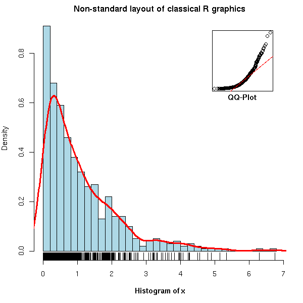
The first part of the book, devoted to the old system, tries to be as complete as a reference book, but fails. For instance, the discussion on how to arrange several plots on a single page sticks to tabular layouts and fails to mention the more flexible "fig" graphical argument (to be honest, it is listed with terser explanations than in the manual page and also appears, deeply hidden in an example, in an appendix).
op <- par(mar = c(5,4,2,2))
N <- 500
x <- rexp(N, 1)
hist(x,
     breaks = 30, probability = TRUE,
     col = "light blue",
     xlab = "",
     main = "Non-standard layout of classical R graphics")
mtext(text = "Histogram of x",
      side = 1, font = 2, line = 3)
lines(density(x),
      col = "red", lwd = 3)
rug(x)
par(new = TRUE,
    fig = c(.7, .9, .7, .9),
    mar = c(0,0,0,0))
qqnorm(x,
       axes = FALSE,
       main = "", xlab = "", ylab = "")
box()
qqline(x,
       col = "red")
par(xpd = NA)
mtext(text = "QQ-Plot",
      line = .2, side = 1, font = 2)
par(op)
On the other hand, the second and largest part, devoted to grid graphics lives up to my expectations: it seems more complete and does not duplicate information already available on the web. You are probably already familiar with some of the high-level lattice plots (xyplot(), histogram(), bwplot()), but if you have already tried to understand how they are implemented, or tried to write your own graphical functions, you were probably confused by the differences (and claimed lack thereof) between "lattice", "panel", "grob" and "grid" -- the book clarifies all that.
The code of the examples in the book is available on the author's web site.
http://www.stat.auckland.ac.nz/~paul/RGraphics/rgraphics.html
You will find, for instance, dendrograms (check the rpart and maptree packages),
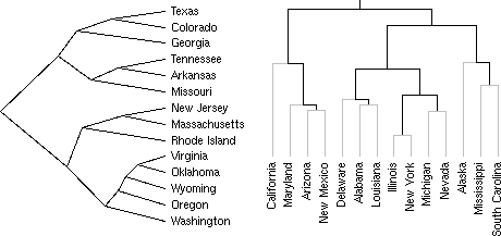
table-like plots

or plots arranged in a tree (this can be seen as a generalization of lattice plots, that present several facets of a dataset arranged on a grid).
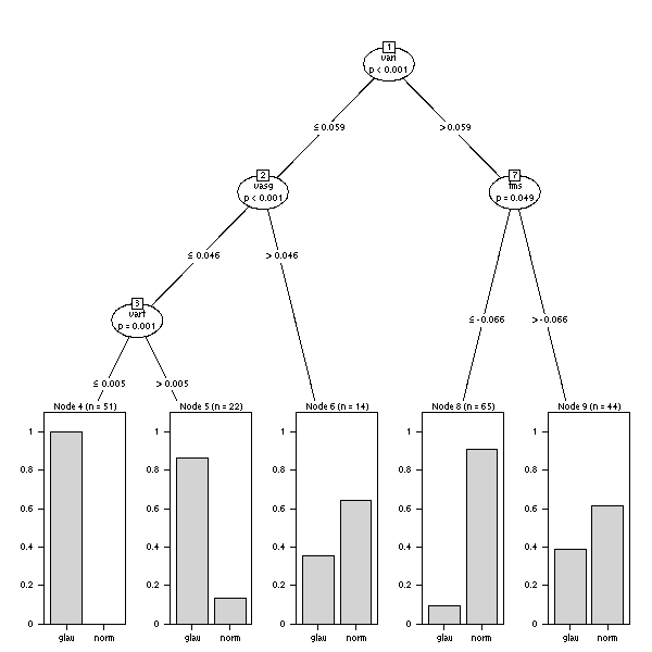
One whole chapter is devoted to the creation, from scratch, of an oceanographic plot
whose elements are then reused for a completely different plot.
The graphical packages (both graphics and grid) do not directly write to the screen or to PDF files, but to an abstraction layer, called grDevices. This helps multiply the number of devices at will: X11, Windows, Quartz, Postscript, PDF, PNG, SVG, GTK, Java, SVG, etc.
It is possible to have several devices at the same time, to switch from one to another (with the dev.list(), dev.cur(), dev.set(), dev.prev(), dev.next(), dev.off(), graphics.off() functions) and to copy data data between them (with the dev.copy() function -- but also check dev.copy2eps(), dev2bitmap(), dev.print(), dev.control()).
R graphics provide little interactivity, but the locator() function (to get the coordinates of a point), the identify() function (to get the name of the point on which you click), the Rggobi package (for the Grand Tour, to visualize high-dimensional datasets, and for brushing), the dynamicGraph and iPlots packages (for real interactivity, in Tcl/Tk or Java) might safisfy your needs.
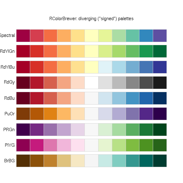
The book contains a very short and insufficient discussion of colours (this is a white and black book), mainly covering rgb(), col2rgb() (to get a colour from its name), hsv(), rgb2hsv(), convertColor(), palette() (to redefine the default palette, i.e., colours 1 (black), 2 (red), 3 (green), etc.), rainbow(), colorRamp(), colorRampPalette() and mentionning the the colorspace and RColorBrewer packages.
library(RColorBrewer)
op <- par(mar = c(2,2,4,2))
display.brewer.all(type = "qual")
mtext(text = "RColorBrewer: qualitative palettes",
side = 3)
par(op)
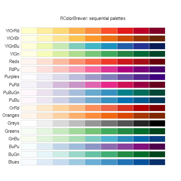
op <- par(mar = c(2,3,4,2))
display.brewer.all(type = "seq")
mtext(text = "RColorBrewer: sequential palettes",
side = 3)
par(op)
op <- par(mar = c(2,2,4,2))
display.brewer.all(type = "div")
mtext(text = 'RColorBrewer: diverging ("signed") palettes',
side = 3)
par(op)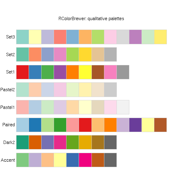
Fonts in R, especially with non-latin1 character sets, are a nightmare -- and the 4-page section devoted to them is neither helpful nor even confident... From time to time, there is an article in RNews that explains how to use one more font, but I always fail to jump to the ceiling screaming "this finally became easy" -- I even fail to think "everything's possible", as I used to in my (La)TeX days...
http://cran.r-project.org/doc/Rnews/Rnews_2006-2.pdf
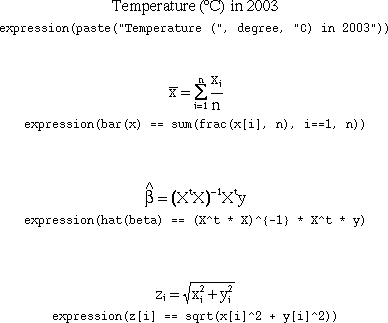
You probably all know that it is possible to add to plots, not only text, but actual mathematical formulas, with greek letters or square roots, but never actually managed to do it: the book clearly explains how to use the expression() and substitute() functions to achieve this. For a finer layout, they can be combined with the strheight(), strwidth(), grobHeight(), grobWidth() functions.
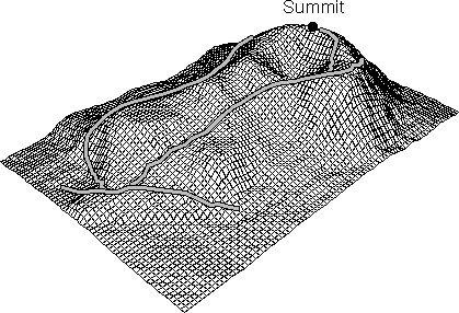
To modify (or "annotate") classical plots, you can use the value they (invisibly) return and extract the coordinates you need: for instance, you can add to a 3-dimensional persp() plot using the quaternion rotation matrix returned by the persp() function.
To create your own plots from scratch, you might need the following functions: plot.new() (to start a new plot), plot.window() (to set the coordinate system), rect(), xycoord() (to accept as argument either two vectors or a 2-column data.frame or matrix), xyzcoord(), n2mfrow() (to find a good number of rows and columns of a multi-plot display in order to have approximately square plots), on.exit() (to reset the graphical parameters, in case the function prematurely ends).
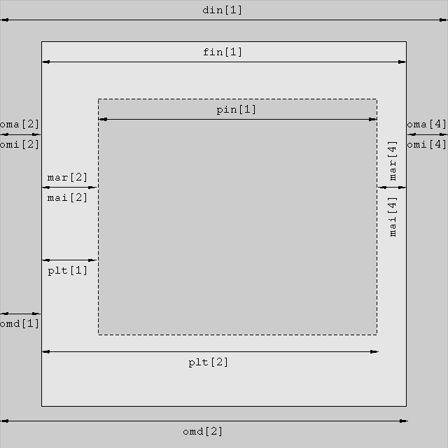
This first part also mentions the generic plot() method (if you create a new class, you can simply provide it with a plot() method), axes, clipping (the "xpd" graphical parameter), text rotation (the "srt" graphical parameter), screen splitting (the mfrow or mfcol graphical parameter, the layout() and split.screen() function), figure dimensions.
The second part of the book starts by tackling the confusion between "lattice", "trellis", "panel", "grob" and "grid".
"Lattice" refers to high-level functions, such as xyplot(), histogram(), bwplot(), splom(), barchart(), densityplot(), dotplot(), qqmath(), qq(), stripplot(), levelplot(), contourplot(), parallel(), cloud() and wireframe().
Most of them are trellis graphics, i.e., they take a cloud of points, cut it into slices, and produce a plot for each slice (we cannot use the word "trellis" because it is a registered trademark, so people use the English translation of that French word -- "lattice").
# From the manual
library(lattice)
Depth <- equal.count(quakes$depth, number = 8, overlap = .1)
xyplot(lat ~ long | Depth, data = quakes)
update(trellis.last.object(),
       strip = strip.custom(strip.names = TRUE,
                            strip.levels = TRUE),
       par.strip.text = list(cex = 0.75),
       aspect = "iso")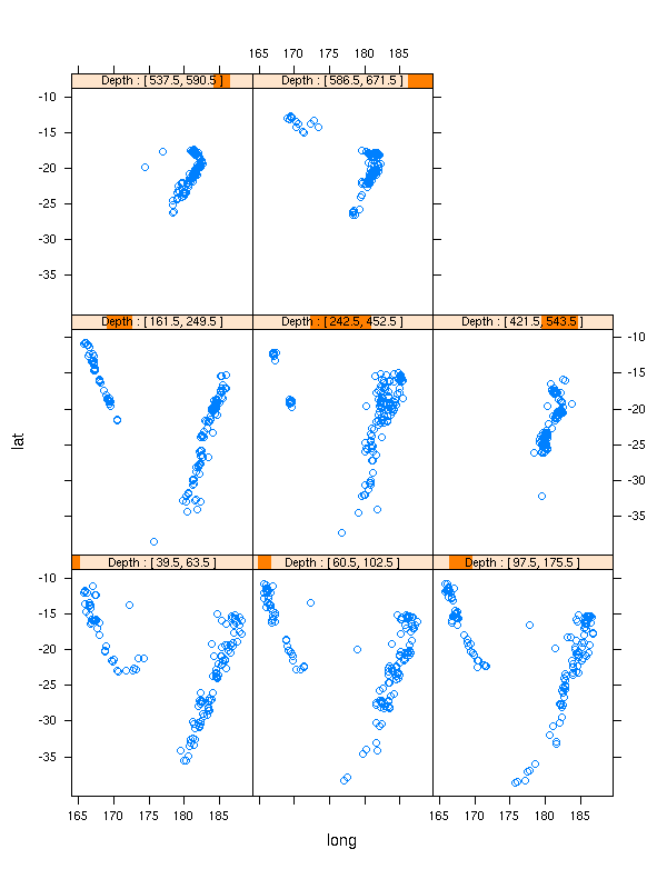
"Panel" refers to the easiest way to configure those functions: the lattice function will split the data (you might also want to use the shingle() or equal.count() function), take care of the axes and other details, and you just provide a "panel" argument, that tells it what to plot (there is also a prepanel argument to set the plot limits, and a strip argument, to display the strip identifying each data slice).
The panel functions you are most likely to use are panel.lmline(), panel.loess(), panel.abline() -- type apropos("panel.*") to have a full list.
xyplot(lat ~ long | Depth, data = quakes,
       panel = function (x, y, ...) {
         panel.xyplot(x, y, ...)
         panel.loess(x, y, col = "blue", lwd = 3, ...)
       },
       strip = strip.custom(strip.names = TRUE,
                            strip.levels = TRUE),
       par.strip.text = list(cex = 0.75),
       aspect = "iso")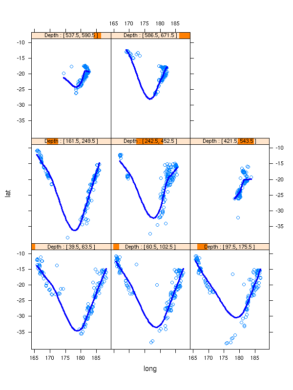
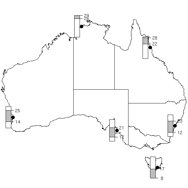
But you can also define your own panel functions: here, a 2-dimensional kernel estimation and a minimum spanning tree.
# Minimum Spanning Tree (MST)
panel.mst <- function (x, y, ...) {
require(ape) # For mst()
d <- dist(cbind(x,y))
m <- mst(d)
i <- which(m == 1)
panel.segments(x[row(m)[i]], y[row(m)[i]],
x[col(m)[i]], y[col(m)[i]],
...)
}
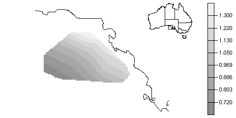
# 2-dimensional Kernel Density Estimation
panel.kde <- function (x, y, ...) {
require(grid) # for convertX() and unit()
require(MASS) # For kde2d()
k <- kde2d(
x, y,
n = 500,
# The limits of the current plot
lims = c(as.numeric(convertX(unit(0,"npc"),"native")),
as.numeric(convertX(unit(1,"npc"),"native")),
as.numeric(convertY(unit(0,"npc"),"native")),
as.numeric(convertY(unit(1,"npc"),"native"))))
panel.levelplot(rep(k$x, length(k$y)),
rep(k$y, each = length(k$x)),
sqrt(k$z),
subscripts = 1:length(k$z),
...)
}
# The same example as above
library(RColorBrewer)
xyplot(lat ~ long | Depth, data = quakes,
panel = function (x, y, ...) {
panel.kde(x, y,
col.regions = brewer.pal(9, "YlOrRd"))
panel.mst(x, y,
col = "black", lwd = 2)
},
strip = strip.custom(strip.names = TRUE,
strip.levels = TRUE),
par.strip.text = list(cex = 0.75),
aspect = "iso")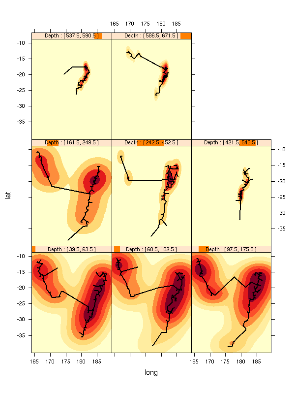
"Grobs" are (low-level) "graphical objects": usually, the plots are not created on the screen, but in memory, arranged in a tree (for instance, a lattice plot is made of several cells, each cell is made of several plots, such as the points and the regression line, in the above example), and only plotted at the end (for instance, lattice plots are only plotted when their print() method is invoked, usually implicitely). After being generated and before being plotted, the plot can be modified: for lattice plots, you can use the update() function.
"Grid" functions do the actual (low-level) plotting.
To complicate things, grobs are typically stored twice: in memory, by the functions that create them, and on the device on which they are plotted, when they are plotted.
To complicate things further, the result of a lattice function is an object of class "trellis", that does not contain any grob yet: they will be created when the object is printed.
The trellis.device() explicitely opens a new plot -- this is the equivalent of the plot.new() (or grid.newpage(), see below) function.
The trellis.par.get(), trellis.par.set() and show.settings() functions are the lattice equivalent of the par() function. To have sensible default values for a given device, you can use the col.whitebg() and canonical.theme() functions. You can also modify those values for a single plot, with the par.settings argument.
It is possible to arrange several lattice plots on a page, either with the layout and aspect arguments, or by explicitely printing them at a given position.
plot1 <- xyplot( y1 ~ x )
plot2 <- xyplot( y2 ~ x )
print(plot1, position = c(0, .2, 1,   1), more = TRUE)
print(plot2, position = c(0,  0, 1, .33), more = TRUE)
You can modify an already-drawn lattice plot with the trellis.focus(), trellis.panelArgs() and trellis.identify() functions.
But if you want a much finer control on your plots, if you want to devise your own plots, you will have to delve deeper, into actual grid functions and grobs.
Grid function plot grobs with respect to the current "viewport", i.e., "drawing context", that contain the limits of the plotting region, the coordinates used (sometimes called the geometric context) and the various graphical parameters (sometimes called the graphical context). You can create a viewport and put it on the display with the pushViewport() function and you can remove it (when you are done) with the popViewport() function (but this is a bad idea: you will not be able to go back to it later). Viewports (as long as you do not pop them) form a hierarchy, through which you can navigate with the upViewport() and downViewport() functions.
# Start a new plot; there is already a default viewport,
# named "ROOT"; create two children viewports, draw a
# frame in each; later revisit them to add some text.
grid.newpage()
grid.rect(gp = gpar(col = "light grey", lwd = 10))
vp1 <- viewport(x = unit(.5,  "npc"),
                y = unit(.25, "npc"),
                width  = unit(.95, "npc"),
                height = unit(.45,  "npc"),
                name = "A")
pushViewport(vp1)
grid.rect(gp = gpar(lwd = 5))
upViewport()
vp2 <- viewport(x = .5,  # npc is actually the default unit
                y = .75,
                width  = .95,
                height = .45,
                name = "B")
pushViewport(vp2)
grid.rect(gp = gpar(lwd = 5))
upViewport()
downViewport("A")
grid.text("Viewport A")
upViewport(0) # Return to the "ROOT" viewport
downViewport("B")
grid.text("Viewport B")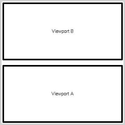
The current.vpTree() function returns the current viewport hierarchy.
> current.vpTree()
viewport[ROOT]->(viewport[A], viewport[B])
By default, viewports clip their contents, but you can set their clip argument to FALSE.
viewport(..., clip = FALSE)
It is possible to push several viewports at the same time, using a vpList().
vp1 <- viewport(width = .9, height = .9, name = "1")
vp2 <- viewport(width = .8, height = .8, name = "2")
vp3 <- viewport(width = .7, height = .7, name = "3")

# Pushing the viewports in parallel
#   viewport[ROOT]->(viewport[1], viewport[2], viewport[3])
grid.newpage()
pushViewport(vpList(vp1, vp2, vp3))
current.vpTree()

# This is equivalent to
grid.newpage()
pushViewport(vp1)
upViewport()
pushViewport(vp2)
upViewport()
pushViewport(vp3)
upViewport()
current.vpTree()

# Pushing the viewports one after the other
#   viewport[ROOT]->(viewport[1]->(viewport[2]->(viewport[3])))
grid.newpage()
pushViewport(vpStack(vp1, vp2, vp3))
current.vpTree()

# This is equivalent to:
grid.newpage()
pushViewport(vp1)
pushViewport(vp2)
pushViewport(vp3)
current.vpTree()
You can go to a viewport by giving its name to the downViewport() function or with (part of) its path.
vpPath("A", "B", "C")Viewports need not be parallel to the axes.
grid.newpage()
grid.rect(gp = gpar(lwd = 10, col = "light grey"))
pushViewport(viewport(
  x = .5, y = .5,
  width = 0.8, height = 0.5,
  angle = 10,
  name = "foo"))
grid.rect(gp = gpar(lwd = 3))
grid.text("A rotated viewport",
          gp = gpar(font = 2,cex = 1.2))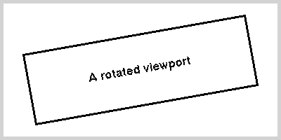
The grid.layout() function helps you define sets of viewports, arranged in a tabular fashion -- to use them in a loop, for instance. In contrast with traditional R graphics, grid layouts can be nested.
grid.newpage()
pushViewport(viewport(
  layout = grid.layout(
    5, 5,
    width  = unit(c(5,1,5,1,5),
                  c("mm", "null", "mm", "null", "mm")),
    height = unit(c(5,1,5,1,5),
                  c("mm", "null", "mm", "null", "mm"))
  ),
  name = "Container"
))
current.vpTree() # Only the containing viewport
for (i in c(2,4)) {
  for (j in c(2,4)) {
    name <- paste("(", i, ",", j, ")", sep = "")
    pushViewport(viewport(layout.pos.row = i,
                          layout.pos.col = j,
                          name =  name))
    grid.rect(gp = gpar(lwd = 3))
    grid.text(name)
    upViewport()
  }
}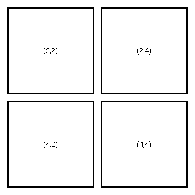
current.vpTree()
# We now have more viewports:
#   viewport[ROOT]->(viewport[Container]->(
#     viewport[(2,2)], viewport[(2,4)],
#     viewport[(4,2)], viewport[(4,4)])
#   )
The grid.frame() and grid.pack() functions provide another way of positioning viewports, similar to the widget packing provided by GUI-building frameworks.
To plot inside a viewport, you can use one of the following functions.
grid.points(), grid.rect(), grid.xaxis(), grid.yaxis(),
grid.text() grid.segments, grid.lines, grid.circle,
grid.arrows(), grid.circle(), grid.polygon();
grid.move.to(), grid.line.to()
It is a good practice to add a "name" argument to those functions: this allows you to revisit and modify the corresponding elements later, with the grid.edit() function.
grid.newpage()
n <- 10
grid.lines(runif(n), runif(n), name = "lines 1")
grid.lines(runif(n), runif(n), name = "lines 2")
grid.edit("lines 1", gp = gpar(col = "red"))
grid.edit("lines 2", gp = gpar(col = "blue"))
grid.edit("lines.*", gp = gpar(lwd = 3),
grep = TRUE, global = TRUE)In traditional graphics, you have a single unit system: the "native" coordinates, fixed by the xlim and ylim arguments of most plotting functions. But when you want to add something (say, a legend, or a thumbnail plot, in a corner) 2mm from the border of the plot, square, 20% as wide as the whole plot, it is next to impossible (it is actually doable, with the "usr" and "fin" graphical parameters). With grid graphics, on the contrary, you can use several units, all at the same time.
n <- 500
x <- rnorm(n)
y <- rnorm(n)
colour <- c(rgb(.8,.2,.2), rgb(1,.8,.8),
            rgb(.5,1,1),   rgb(.8,1,1))
grid.newpage()
pushViewport(viewport(
  layout = grid.layout(
    3, 3,
    width  = unit(c(5,1,5),
                  c("mm", "null", "mm")),
    height = unit(c(15,1,5),
                  c("mm", "null", "mm"))
  ),
  name = "Container"
))
pushViewport(viewport(
  layout.pos.row = 2,
  layout.pos.col = 2,
  xscale = range(x) + .1 * c(-1,1) * diff(range(x)),
  yscale = range(y) + .1 * c(-1,1) * diff(range(y)),
  name =  "Main plotting area"
))
upViewport()
pushViewport(viewport(
  layout.pos.row = 1,
  layout.pos.col = 2,
  name =  "Title"
))
upViewport()
downViewport("Main plotting area")
grid.rect(gp = gpar(lwd = 3, fill = colour[2]))
grid.points(x, y, pch = 16, gp = gpar(col = colour[1]))
grid.points(x, y, pch = 1)
# The specification of the thumbnail is straightforward:
# 5mm from the upper right corner, 25% of the picture
# height and width
pushViewport(viewport(
  x = unit(1, "npc") - unit(5, "mm"),
  y = unit(1, "npc") - unit(5, "mm"),
  width  = .25 * unit(1, "npc"),
  height = .25 * unit(1, "npc"),
  xscale = range(x) + .1 * c(-1,1) * diff(range(x)),
  yscale = range(y) + .1 * c(-1,1) * diff(range(y)),
  just = c("right", "top")
))
grid.rect(gp = gpar(lwd = 3, fill = colour[4]))
grid.points(sort(x), sort(y),
            pch = 16, gp = gpar(cex = .5))
upViewport(0)
downViewport("Title")
grid.text("Thumbnail in a grid plot",
          gp = gpar(font = 2, cex = 1.2))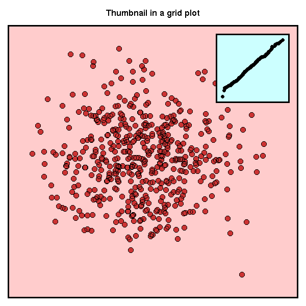
Here are some of the units available (they can be used whenever a number is expected).
unit(100, "native")   # User-defined coordinates (xlim, ylim)
unit(.8,  "npc")      # Normalized Parent Coordinates
unit(.8,  "snpc")     # Squared npc
unit(1,   "mm")
unit(1,   "cm")
unit(1,   "points")
unit(1,   "char")     # Current character size
unit(1,   "lines")    # Current lineheight
                      # (for the current font)
The following units are useful in grid.layout():
unit(1,   "null")     # Spring ("glue", \hfill or \hss
                      # in TeX)
unit(1,   "grobwidth")# The viewport will take the width
                      # of its contents
The unit() function can also return the dimensions of an object:
  unit(1, "strwidth", "some text")
  unit(1, "grobwidth", textGrob("some text"))
The convertX() and convertY() functions perform conversions between those units. For instance, the following computes the horizontal and vertical limits of the drawing area.
xlim <- convertX(unit(0:1, "npc"), "native", valueOnly = TRUE)
ylim <- convertY(unit(0:1, "npc"), "native", valueOnly = TRUE)
There is a grid.locator() function, for very simple interactive use.
The grid.get() function gets an object from its name; grid.edit() changes some of the atributes of an object identified by its name (including the graphical context gp); grid.remove() deletes it from the display; grid.add() adds an object (to an already existing object, typically a gList); grid.set() replaces an object; grid.newpage() starts a new plot; getNames() gives the names of all the objects; childNames() gives the names of the children of an object.
When specifying an object name, you can also add the grep=TRUE argument to query for a regular expression instead of an exact name or the global=TRUE argument to retrieve all the corresponding objects, not only the first.
Instead of specifying a name, you can give a path, e.g., gPath("foo", "bar").
The graphical parameters are given as a gpar object in the gp argument -- there are a few exceptions, though, such as the "pch" argument of grid.points().
The get.par() function returns the default value of those parameters.
Grid functions can also be given a viewport as a vp argument.
You can use grid functions inside a panel function -- it allows you to use coordinates other than "native". Conversely, one can use lattice functions inside grid graphics: just make sure to call the print() method on the result of the lattice or panel function.
n <- 500
x <- rexp(n,1)
colour <- c(rgb(.5,1,1),   rgb(.8,1,1),
            rgb(.8,.2,.2), rgb(1,.8,.8))

grid.newpage()
pushViewport(viewport(
  layout = grid.layout(
    3, 3,
    width  = unit(c(5,1,5),
                  c("mm", "null", "mm")),
    height = unit(c(15,1,5),
                  c("mm", "null", "mm"))
  ),
  name = "Container"
))
pushViewport(viewport(
  layout.pos.row = 2,
  layout.pos.col = 2,
  xscale = range(x) + .1 * c(-1,1) * diff(range(x)),
  yscale = c(-.05,1),
  name =  "Main plotting area"
))
upViewport()
pushViewport(viewport(layout.pos.row = 1,
                      layout.pos.col = 2,
                      name =  "Title"))
upViewport()
# Histogram
downViewport("Main plotting area")
grid.rect(gp = gpar(lwd = 3, fill = colour[2]))
print(panel.histogram(x,
  breaks = seq(from = min(x), to = max(x),
               #length = nclass.Sturges(x)
               length = 20
)))
print(panel.axis(side = "bottom")) # Not what I wanted
# qq-plot
y <- qnorm(ppoints(length(x)))
pushViewport(viewport(
  x = unit(1, "npc") - unit(5, "mm"),
  y = unit(1, "npc") - unit(5, "mm"),
  width  = .25 * unit(1, "npc"),
  height = .25 * unit(1, "npc"),
  xscale = range(y) + .1 * c(-1,1) * diff(range(y)),
  yscale = range(x) + .1 * c(-1,1) * diff(range(x)),
  just = c("right", "top")
))
grid.rect(gp = gpar(lwd = 3, fill = colour[4]))
grid.points(y, sort(x),
            pch = 16,
            gp = gpar(cex = .5))
yy <- quantile(x[!is.na(x)], c(0.25, 0.75))
xx <- qnorm(c(0.25, 0.75))
slope <- diff(yy)/diff(xx)
int <- yy[1] - slope * xx[1]
# Why is there no grid.abline?
# (because there would be a unit problem for the slope:
# its unit is a ratio of two units, a vertical and a
# horizontal one...)
print(panel.abline(int, slope,
                   col = "red", lwd = 2))
# Title
upViewport(0)
downViewport("Title")
grid.text("Panel thumbnail in a grid plot",
          gp = gpar(font = 2, cex = 1.2))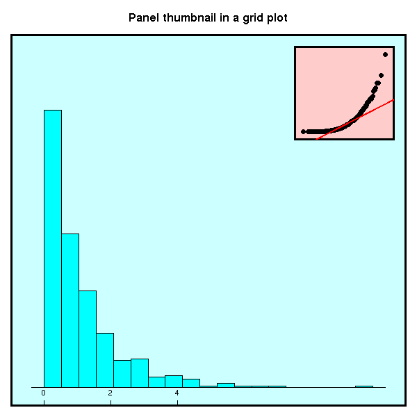
Instead of drawing directly on the screen, with the grid.*() functions, we can build graphical objects, combine them, modify them, create a whole scene off-screen, and only plot it when it is finished. Those graphical objects are called "grobs".
Here are the grob equivalents of the functions mentionned above.
linesGrob(), segmentsGrob(), rectGrob(), circleGrib(),
polygonGrob(), textGrob(), arrowsGrob(), pointsGrob(),
xaxisGrob(), yaxisGrob();
moveToGrob(), lineToGrob();
getGrob(), editGrob(), addGrob(), removeGrob(), setGrob();
frameGrob(), placeGrob().
Grobs can be "combined" (or "grouped") to form larger, hierarchical grobs or gTrees.
grobC <- gTree(children=gList(grobA, grobB))
grid.draw(grobC)
The grid.grab() function captures all the currently displayed grobs, e.g., the result of a lattice plot.
histogram(x)
scene <- grid.grab()

# To look at the contents
childNames(scene)
# To see what an element is, if its name is not explicit
# enough, you can change its colour.
grid.newpage()
grid.draw(scene)
grid.edit(scene$children[[3]]$name,
          gp = gpar(col = "red"))
The grid.grabExpr() function does the same thing, off-screen.
scene <- grid.grabExpr( print(histogram(x)) )
The last chapter explains how to develop new graphical functions, stressing good programming practices, such as modularity -- lattice functions, though impressive, are not that flexible.
The simplest way of writing such a function is is to use the grid.* functions: write a function for each of the components of your plot, then write a function that parses the data to be plotted, sets up the viewports and calls the previous functions. In order to facilitate the annotation of your plot, prefer upViewport() to popViewport() (the latter destroys the viewport...) and be sure to name all the elements -- using named elements relieves you from the need to provide an explosive number of arguments to configure the plot.
But that is not as reuseable as it could get: it is also possible to define new types ("classes" -- actually S3 classes) of grobs. You first need a constructor, i.e., a function that returns an instance of your class.
myGrob <- function (foo, bar,
                    name = NULL, gp = NULL, vp = NULL) {
  # Always inherit from gTree() -- the S3 object-oriented
  # paradigm is too limited: it does not allow structure
  # (slots) inheritance.
  res <- gTree(foo = foo,      # The slots my object needs
               bar = bar,
               name = name,    # The slots of a gTree
               gp = gp,
               vp = vp,
               children = gList(makeMyGrob(foo, bar)),
               cl = "myGrob"   # The name of the class
              )
  res
}
You should also provide a validDetail() method, to check that the slots of the object have valid values: it will be called when the object is created or modified -- the gp, vp, name, children and childrenvp slots are always (implicitely) checked.
validDetails.myGrob <- function (x) {
  if (! all(x$foo < 0) | ! all(x$bar > 0)) {
    stop("foo and bar should be positive")
  }
  x   # Always return the object -- you might
      # even want to modify it before
}
You may want to provide a drawDetails() method, if the drawing is not straightforward (if there are computations to do, e.g., positions or distances that depend on quantities only known when the plot is actually drawn, or if you want to have a single object in spite of a large number of components (e.g., axis ticks). For completeness, you should provide a grid.myGrob() function.
grid.myGrob <- function (...) {
  grid.draw(myGrob(...))
}
You should provide an editDetails() method if changes in the values of the slots should result in changes in the children of the gTree -- this is almost always the case: the children, or even their number can change.
# More examples in the book, including: adding a grob to
# the list of children, propagating graphical parameters
# to the children, modifying the childrenvp slot.

editDetails.myGrob <- function (x, specs) {
  if ( "foo" %in% names(specs) || "bar %in% names(specs) ){
    x <- setChildren(x, makeMyGrob(x$foo, x$bar)
  }
  x
}
You may also (rarely) want to provide widthDetails(), heightDetails(), preDrawDetails() (to push viewports) and postDrawDetails() methods.
I feel that here, I should give an actual example, different from that in the book -- but I am not skilled enough yet...
The book ends with a multi-way example: how to write a grid.*() function or define a new grob class, reusing already-defined grid.*() functions or grobs. An appendix explains how to use grid graphics inside a traditional plot (using the gridBase package) or how to use classical graphics inside a grid plot (using the "fig" or "plt" graphical argument).
posted at: 19:18 | path: /R | permanent link to this entry
