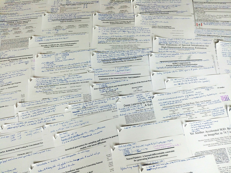
Rather than a review of 2019 in machine learning, this is a review of (some of) what I read this year: this is biased towards my interests, incomplete, and some of the topics may already be a few years old.
1a. The main transformation in the machine learning landscape was undoubtedly the rise of language models: they are not only more powerful, trained on more data, they are also more directly usable, thanks to the HuggingFace transformers library.
https://huggingface.co/transformers/index.html
It is difficult, however, to keep track of which model is currently the best. When you read this, it may no longer be one of the following: BERT and its many variants (Albert (lightweight), RoBERTa (Facebook), DistilBERT, CamemBERT (French), Ernie (Baidu, Chinese), etc.), XLNet, XLM, GPT-2, etc.).
1b. Those models provide contextual word embeddings – in contrast to word2vec, GloVe, FastText, which are not contextual.
Visualizing and measuring the geometry of BERT
https://arxiv.org/abs/1906.02715

Contextual string embeddings for sequence labelings
https://pdfs.semanticscholar.org/421f/c2556836a6b441de806d7b393a35b6eaea58.pdf
1c. There has also been some work on multilingual models, in particular multilingual embeddings: for languages with less training data, one can simply learn a single model for several (related) languages.
Image search using multilingual texts: a cross-modal learning approach between image and text
https://arxiv.org/abs/1903.11299

https://github.com/facebookresearch/MUSE
1d. Some (traditional) word embeddings can account for polysemy.
Linear algebraic structure of word senses with applications to polysemy
https://arxiv.org/abs/1601.03764

Multimodal word distributions
https://arxiv.org/abs/1704.08424
2. "Self-supervised learning" is a special case of unsupervised learning (or a first, pretraining, step in semi-supervised learning, or pre-training for supervised learning) in which we turn the unlabeled data into a supervised problem. For instance, given unlabeled images, we can train a model to tell if two patches come from the same image. Given sound data, we can train a model to tell if two patches are close in time or not – the features learned will identify phonemes, if we want very close patches, or speakers, for slightly more distant ones.
posted at: 11:36 | path: /R | permanent link to this entry
Many problems in statistics or machine learning are of the form "find the values of the parameters that minimize some measure of error". But in some cases, constraints are also imposed on the parameters: for instance, that they should sum up to 1, or that at most 10 of them should be non-zero -- this adds a combinatorial layer to the problem, which makes it much harder to solve.
In this note, I will give a guide to (some of) the optimization packages in R and explain (some of) the algorithms behind them. The solvers accessible from R have some limitations, such as the inability to deal with binary or integral constraints (in non-linear problems): we will see how to solve such problems.
When you start to use optimization software, you struggle to coax the problem into the form expected by the software (you often have to reformulate it to make it linear or quadratic, and then write it in matrix form). This is not very user-friendly. We will see that it is possible to specify optimization problems in a perfectly readable way.
# Actual R code
x <- variable(5)
minimize( sum(abs(x)) + sum(x^2) - .2*x[1]*x[2] )
x >= 0
x <= 1
sum(x) == 1
x[1] == x[2]
r <- solve()
Many of the examples will be taken from finance and portfolio optimization.
posted at: 19:18 | path: /R | permanent link to this entry
I did not attend the conference this year, but just read through the presentations. There is some overlap with other R-related conferences, such as R in Finance or the Rmetrics workshop.
http://www.agrocampus-ouest.fr/math/useR-2009/
http://www.rinfinance.com/
http://www.rmetrics.org/meielisalp.htm
Here are some more detailed notes.
posted at: 19:18 | path: /R | permanent link to this entry
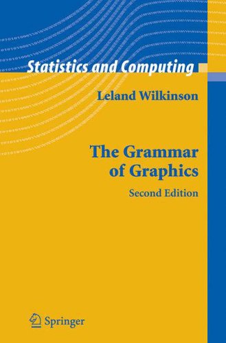
Though this book is supposed to be a description of the graphics infrastructure a statistical system could provide, you can and should also see it as a (huge, colourful) book of statistical plot examples.
The author suggests to describe a statistical plot in several consecutive steps: data, transformation, scale, coordinates, elements, guides, display. The "data" part performs the actual statistical computations -- it has to be part of the graphics pipeline if you want to be able to interactively control those computations, say, with a slider widget. The transformation, scale and coordinate steps, which I personnally view as a single step, is where most of the imagination of the plot designer operates: you can naively plot the data in cartesian coordinates, but you can also transform it in endless ways, some of which will shed light on your data (more examples below). The elements are what is actually plotted (points, lignes, but also shapes). The guides are the axes, legends and other elements that help read the plot -- for instance, you may have more than two axes, or plot a priori meaningful lines (say, the first bissectrix), or complement the title with a picture (a "thumbnail"). The last step, the display, actually produces the picture, but should also provide interactivity (brushing, drill down, zooming, linking, and changes in the various parameters used in the previous steps).
In the course of the book, the author introduces many notions linked to actual statistical practice but too often rejected as being IT problems, such as data mining, KDD (Knowledge Discovery in Databases); OLAP, ROLAP, MOLAP, data cube, drill-down, drill-up; data streams; object-oriented design; design patterns (dynamic plots are a straightforward example of the "observer pattern"); eXtreme Programming (XP); Geographical Information Systems (GIS); XML; perception (e.g., you will learn that people do not judge quantities and relationships in the same way after a glance and after lengthy considerations), etc. -- but they are only superficially touched upon, just enough to wet your apetite.
If you only remember a couple of the topics developped in the book, these should be: the use of non-cartesian coordinates and, more generally, data transformations; scagnostics; data patterns, i.e., the meaningful reordering of variables and/or observations.
posted at: 19:18 | path: /R | permanent link to this entry
I have just uploaded the new version of my "Statistics with R":
http://zoonek2.free.fr/UNIX/48_R/all.html
The previous version was one year and a half old, so in spite of the fact I have not had much time to devote to it in the past two years, it might have changed quite a bit -- but it remains as incomplete as ever.
posted at: 19:18 | path: /R | permanent link to this entry
I just finished reading Paul Murrel's book, "R graphics".
There are two graphical systems in R: the old ("classical" -- in the "graphics" package) one, and the new ("trellis", "lattice", "grid" -- in the "lattice" and "grid" packages) one.
The first part of the book, devoted to the old system, tries to be as complete as a reference book, but fails. For instance, the discussion on how to arrange several plots on a single page sticks to tabular layouts and fails to mention the more flexible "fig" graphical argument (to be honest, it is listed with terser explanations than in the manual page and also appears, deeply hidden in an example, in an appendix).
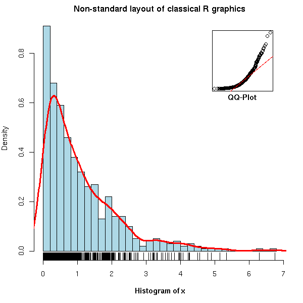
op <- par(mar = c(5,4,2,2))
N <- 500
x <- rexp(N, 1)
hist(x,
     breaks = 30, probability = TRUE,
     col = "light blue",
     xlab = "",
     main = "Non-standard layout of classical R graphics")
mtext(text = "Histogram of x",
      side = 1, font = 2, line = 3)
lines(density(x),
      col = "red", lwd = 3)
rug(x)
par(new = TRUE,
    fig = c(.7, .9, .7, .9),
    mar = c(0,0,0,0))
qqnorm(x,
       axes = FALSE,
       main = "", xlab = "", ylab = "")
box()
qqline(x,
       col = "red")
par(xpd = NA)
mtext(text = "QQ-Plot",
      line = .2, side = 1, font = 2)
par(op)
On the other hand, the second and largest part, devoted to grid graphics lives up to my expectations: it seems more complete and does not duplicate information already available on the web. You are probably already familiar with some of the high-level lattice plots (xyplot(), histogram(), bwplot()), but if you have already tried to understand how they are implemented, or tried to write your own graphical functions, you were probably confused by the differences (and claimed lack thereof) between "lattice", "panel", "grob" and "grid" -- the book clarifies all that.
The code of the examples in the book is available on the author's web site.
http://www.stat.auckland.ac.nz/~paul/RGraphics/rgraphics.html
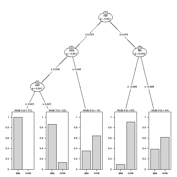
You will find, for instance, dendrograms (check the rpart and maptree packages),
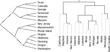
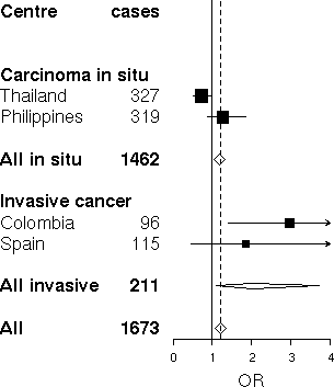
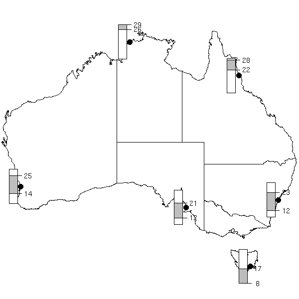
table-like plots
or plots arranged in a tree (this can be seen as a generalization of lattice plots, that present several facets of a dataset arranged on a grid).
One whole chapter is devoted to the creation, from scratch, of an oceanographic plot
whose elements are then reused for a completely different plot.
posted at: 19:18 | path: /R | permanent link to this entry
Last week, I attended the 2006 UseR! conference: here is a (long) summary of some of the talks that took place in Vienna -- since there were up to six simultaneous talks, I could not attend all of them...
In this note:
0. General remarks
1. Tutorial: Bayesian statistics and marketing
2. Tutorial: Rmetrics
3. Recurring topics
4. Other topics
5. Conclusion
For more information about the contents of the conference and about the previous ones (the useR! conference was initially linked to the Directions in Statistical Computing (DSC) ones):
http://www.r-project.org/useR-2006/
http://www.ci.tuwien.ac.at/Conferences/useR-2004/
http://www.stat.auckland.ac.nz/dsc-2007/
http://depts.washington.edu/dsc2005/
http://www.ci.tuwien.ac.at/Conferences/DSC-2003/
http://www.ci.tuwien.ac.at/Conferences/DSC-2001/
http://www.ci.tuwien.ac.at/Conferences/DSC-1999/
I attended two tutorials prior to the conference: one on bayesian statistics (in marketing) and one on Rmetrics.
There were 400 participants, 160 presentations.
Among the people present, approximately 50% were using Windows (perhaps less: it is very difficult to distinguish between Windows and Linux), 30% MacOS, 20% Linux (mostly Gnome, to my great surprise).
posted at: 19:18 | path: /R | permanent link to this entry
