Many problems in statistics or machine learning are of the form "find the values of the parameters that minimize some measure of error". But in some cases, constraints are also imposed on the parameters: for instance, that they should sum up to 1, or that at most 10 of them should be non-zero -- this adds a combinatorial layer to the problem, which makes it much harder to solve.
In this note, I will give a guide to (some of) the optimization packages in R and explain (some of) the algorithms behind them. The solvers accessible from R have some limitations, such as the inability to deal with binary or integral constraints (in non-linear problems): we will see how to solve such problems.
When you start to use optimization software, you struggle to coax the problem into the form expected by the software (you often have to reformulate it to make it linear or quadratic, and then write it in matrix form). This is not very user-friendly. We will see that it is possible to specify optimization problems in a perfectly readable way.
# Actual R code
x <- variable(5)
minimize( sum(abs(x)) + sum(x^2) - .2*x[1]*x[2] )
x >= 0
x <= 1
sum(x) == 1
x[1] == x[2]
r <- solve()
Many of the examples will be taken from finance and portfolio optimization.
Optimization refers to the problem of finding the minimum or the maximum of some function, subject to a few constraints. Optimization problems (sometimes called "optimization programs" -- the word comes from an era with no computers and no computer programs) are often written as
Find         x
To maximize  f(x)
Such that    g(x)  = 0
and          h(x) >= 0
where x is a vector and f, g, h arbitrary functions.
Let us first describe some of the complications that can occur when you are faced with an optimization problem.
Since many optimization algorithms only use local information, they can get stuck in a local extremum. In the following example, there are many valleys: the computer will find one of them, but not necessarily the lowest.
# Optimization problem with many extrema: non-linear regression
#   y = sin( a * x + b ) + noise
n <- 100
x <- seq(0,1,length=n)
f <- function(x,a,b) sin(a*x+b)
y <- f(x, 4*pi*runif(1), 2*pi*runif(1)) + rnorm(n)
g <- function(a,b) sum((f(x,a,b) - y)^2)
N <- 200
a <- seq(0, 10*pi, length=N)
b <- seq(0,  2*pi, length=N)
z <- outer(a, b, Vectorize(g))
image(a, b, z,
  las=1,
  main="Multiple extrema",
  xlab="Frequency",
  ylab="Phase"
)
# Compute the extrema visible on the plot
shift <- function(z,i,j) {
  n <- nrow(z)
  m <- ncol(z)
  u <- NA * z
         if(i >= 0  && j >= 0) { u[1:(n-i),  1:(m-j)] <- z[(i+1):n, (j+1):m]
  } else if(i <= 0  && j >= 0) { u[(-i+1):n, 1:(m-j)] <- z[1:(n+i), (j+1):m]
  } else if(i >= 0  && j <= 0) { u[1:(n-i), (-j+1):m] <- z[(i+1):n, 1:(m+j)]
  } else if(i <= 0  && j <= 0) { u[(-i+1):n,(-j+1):m] <- z[1:(n+i), 1:(m+j)]
  }
  u
}
u <- v <- z == z
for(i in c(-1,0,1))
for(j in c(-1,0,1))
if(abs(i)+abs(j)>0) {
  tmp <- shift(z,i,j)
  u <- u & z >= tmp
  v <- v & z <= tmp
}
v <- which(v, arr.ind=TRUE )
v <- t(apply(v,1,function(u) c(a[u[1]], b[u[2]])))
v <- t(apply(v, 1, function(r) optim(r, function(p) g(p[1],p[2]))$par))
points(v, pch="+", cex=2)
u <- which(u, arr.ind=TRUE )
u <- t(apply(u,1,function(u) c(a[u[1]], b[u[2]])))
u <- t(apply(u, 1, function(r) optim(r, function(p) -g(p[1],p[2]))$par))
points(u, pch="-", cex=2)
# Not much to see on the 3D plot
library(rgl)
persp3d(a,b,z)
(In this example, you could use a more robust optimization algorithm, such as DEoptim, or, better, get rid of the waves and local extrema by expanding the sine.)
The situation is often made more complicated by the presence of constraints. Fortunately, they can often be removed by reformulating the problem: if you have an equality constraint, you can often express one of the unknowns as a function of the others; if you have an inequality constraint of the form x>=0, you can replace x with exp(y) or y^2 or log(1+exp(y)), where y is a new unknown.
For instance, let us consider a constrained regression:
y = a * x1 + b * x2 + c * x3 + noise
a + b + c = 1
a, b, c >= 0.
The problem can be reparametrized as follows.
# Parameters
k <- 3
a <- diff(c(0, sort(runif(k-1)), 1))
# Data
n <- 1e4
x <- matrix(rnorm(k*n), nc=k)
y <- x %*% a + rnorm(n)
# Log-Likelihood
f <- function(u) sum((y - x %*% u)^2)
# Transform the parameters: we just have
# to find a bijection between R^2
# and {(a,b,c) \in [0,1]^3 : a+b+c=1}.
g <- function(v) {
  # Ensure they in [0,1]
  v <- 1/(1+exp(-v))
  # Ensure they add up to 1
  v <- c( v[1], v[2] * (1-v[1]) )
  u <- c(v, 1-sum(v))
  u
}
# Minimize the log-likelihood
r <- optim( rnorm(k-1), function(v) f(g(v)) )
g( r$par ); a  # Reasonably similar
Unfortunately, this approach does not always work. Consider the following problem. Given n numbers a[1],...,a[n], we want to find x1,...,xn, as close as possible from the a[i], but in increasing order. If we use the sum of the squared distances to measure closeness, the optimization problem can be written as
Find        x1,...,xn
to minimize sum( (a-x)^2 )
such that   x1 <= x2 <= ... <= xn.
Instead of looking for x1,x2,...,xn, we can look for
y1 = x1
y2 = x2 - x1
...
yn = xn - x[n-1]
The problem becomes
Find        y1,...,yn
to minimize sum( (a-cumsum(y))^2 )
such that   y >= 0
The constraint is simpler, but we have not completely gotten rid of it. But we can write y = exp(z): that will ensure it remains positive. The constraints have now completely disappeared:
Find        z1,...,zn
to minimize sum( (a-cumsum(exp(z)))^2 )
and return  x = cumsum(exp(z)).
In code:
# 20 numbers, in increasing order,
# but 5 of them have been shuffled.
n <- 20
a0 <- a <- round(100*sort(runif(n)))
i <- sample(n, 5)
a[i] <- sample(a[i])
plot(a, type="b", las=1)
# Objective
f <- function(u) sum( (a-cumsum(exp(u)))^2 )
r <- optim(0*a, f)
x <- cumsum(exp(r$par))
lines(x, lwd=3, col="navy")
f(r$par)
f(c(log(a0[1]), log(diff(a0))))  # Much lower
We have a very bad solution. One of the problems is that the solution is on the frontier, but the frontier is no longer reachable after our reparametrization. In this case, quadratic programming is a better approach.
# Correct solution with quadprog
library(quadprog)
A <- -diag(n)[-n,] + cbind(0,diag(n-1))
r <- solve.QP(diag(n), a, t(A), rep(0,n-1))
x <- r$solution
plot(a, type="b", lwd=3, las=1)
lines(x, lwd=3, col="navy")
In some cases, the constraints are too irregular or too numerous: we cannot remove them. Instead, we can add a penalty for constraint breaches, and progressively increase the penalty.
# Same example
n <- 20
a0 <- a <- round(100*sort(runif(n)))
i <- sample(n, 5)
a[i] <- sample(a[i])
plot(a, type="b", las=1)
x <- a
for(penalty in c(1,5,10,50,100,1e3,1e4,1e5,1e6,1e7,1e8,1e9)) {
  # Use a smooth penalty, e.g., pmax(x,0)^2,
  # rather than a merely continuous one, such as pmax(x,0):
  # otherwise, the frontier of the feasibility region
  # becomes "sticky": once you reach it, the algorithm
  # (Nelder-Mead, here) refuses to leave it.
  f <- function(u) sum( (a-u)^2 ) + penalty * sum(pmax(-diff(u),0)^2)
  # Increase the number of iteration:
  # with the default 500, it does not converge...
  r <- optim(x, f, control=list(maxit=1e4))
  x <- r$par
}
lines(x, lwd=3, col="navy")
f(x)
A <- -diag(n)[-n,] + cbind(0,diag(n-1))
r <- solve.QP(diag(n), a, t(A), rep(0,n-1))
y <- r$solution
f(y)The functions to solve optimization problems are scattered in many packages, each limited to (or optimized for) problems of a certain type. To complicate things, the interfaces are different.
Here are some of them.
|-----------------+-----------+-----------+-------------+---------------|
|                 | Linear    | Quadratic | Non-linear  | badly-behaved |
|                 | objective | objective | objective   | objective     |
|-----------------+-----------+-----------+-------------+---------------|
| No constraints, |           |           | optim       | DEoptim       |
| Box constraints |           |           | optimize    | rgenoud       |
|                 |           |           | nlminb      | NMOF          |
|                 |           |           |             | psoptim       |
|-----------------+-----------+-----------+-------------+---------------|
| Linear          |           | quadprog  | constrOptim |               |
| constraints     |           |           |             |               |
|-----------------+-----------+-----------+-------------+---------------|
| Linear, integer | Rglpk     |           |             |               |
| constraints     | lpSolve   |           |             |               |
|                 | Rsymphony |           |             |               |
|-----------------+-----------+-----------+-------------+---------------|
| Quadratic       |           |           |             |               |
|-----------------+-----------+-----------+-------------+---------------|
| Semi-definite   | Rcsdp     |           |             |               |
|-----------------+-----------+-----------+-------------+---------------|
| Non-linear      |           |           | Rsolnp      |               |
| constraints     |           |           | alabama     |               |
|-----------------+-----------+-----------+-------------+---------------|
There have been a few attempts to unify all those packages, e.g. the ROI and optimx packages (they allow you to first describe the optimization problem, always in the same way, regardless of the type of the problemm and only then to select the solver to use, ROI for mathematical programming, optimx for optimization with no or box constraints), but they are still incomplete and lack documentation.
There is a more exhaustive list in the Optimization task view.
http://cran.r-project.org/web/views/Optimization.html
If you are unfamiliar with them, I suggest to check them in the following order. Optim will be sufficient for most of your optimization needs, but you may want to resort to DEoptim for problems with many local extrema. For non-linear problems with non-box constraints (i.e., constraints specified by several functions, with equalities or inequalities, rather than upper and lower bounds), use Rsolnp. If the problem is large, and linear or quadratic, you will want to try Rglpk or quadprog instead: they will be much faster, but it can be tricky to write the problem in matrix form.
Some of those solvers have limitations. For instance, lpSolve imposes that all the variables be non-negative (it is in the documentation, with an exclamation mark, but it is easy to overlook -- Rglpk as the same default behaviour, but it can be changed); quadprog only works for strictly convex problems (the quadratic form must be positive definite, but if you have to add slack variables to transform some of the constraints, you end up with a positive semi-definite matrix and it no longer works -- this is a serious limitation); integrality constraints can only be imposed on some of the linear solvers.
Except for the non-linear solvers (and Rglpk, to which you can give a text file), it is not possible to specify the problems in a human-readable way: just matrices.
If your problem is not linear but can easily be converted into a linear problem you have to make the transformation yourself. Some of the transformations (e.g., separating the positive and negative value of a number to express its absolute value) are easy, but other are more complex, time-consuming, and error-prone (e.g., converting the expected shortfall into a linear quantity, or converting quadratic constraints into semi-definite constraints).
Linear regression is an optimization problem: we are looking for the value of b that minimizes the residual sum of squares.
RSS = ( Y - X b )' ( Y - X b )
    = Y Y' - 2 Y' X b + b X' X b
Let us compare the optimization problem with the regression.
# Sample data
n <- 100
x1 <- rnorm(n)
x2 <- rnorm(n)
y <- 1 + x1 + x2 + rnorm(n)
X <- cbind( rep(1,n), x1, x2 )

# Regression
r <- lm(y ~ x1 + x2)

# Optimization
library(quadprog)
s <- solve.QP( t(X) %*% X, t(y) %*% X, matrix(nr=3,nc=0), numeric(), 0 )
coef(r)
s$solution  # Identical
The reformulation of the regression problem as an optimization problem allows you to easily add linear constraints. For instance, you may want the coefficients of the regression to sum up to 1.
# Sample data
n <- 100
x1 <- rnorm(n)
x2 <- rnorm(n)
x3 <- rnorm(n)
y <- .3 * x1 + .2 * x2 + .5*x3 + rnorm(n)
X <- cbind( x1, x2, x3 )

# No constraints
r <- lm(y ~ x1 + x2 + x3 - 1)
coef(r)
sum(coef(r))

# The coefficients should sum up to 1
library(quadprog)
s <- solve.QP( t(X) %*% X, t(y) %*% X, matrix(1, nr=3, nc=1), 1, meq=1 )
s$solution
sum(s$solution)

# Also ask that the coefficients be in [0,1]
s <- solve.QP(
  t(X) %*% X, t(y) %*% X,
  cbind(  # One constraint per COLUMN
    matrix(1, nr=3, nc=1),
    diag(3),
    -diag(3)
  ),
  c(1, 0,0,0, -1,-1,-1),
  meq = 1 # Only the first constraint is an equality, the others are >=
)
s$solution
sum(s$solution)

# Comparison with mgcv::pcls
library(mgcv)
M <- list(
  X = X, y = y,
  p = rep(1/3,3),       # A feasible solution
  w = rep(1,length(y)), # weights
  Ain = rbind(diag(3),-diag(3)),  # Inequality constraints
  bin = c(rep(0,3), rep(-1,3)),
  C = matrix(1, nc=3, nr=1), # Equality constraints, one constraint per ROW
  off=array(0,0), S=list(), sp=array(0,0)
)
pcls(M)

# Comparison with limSolve::lsei
library(limSolve)
lsei(
  A=X, B=y,
  E = matrix(1, nc=3, nr=1), F = 1, # Equality constraints
  G = diag(3), H = rep(0,3),        # Inequalities
  type=1                            # lsei (you can also use quadprog)
)$XThe problem of finding the median of a set of numbers x1,...xn can be formulated as a non-linear optimization problem:
Find mu
to minimize sum( abs( x[i] - mu ) ).
It can be reformulated as a linear problem, by replacing the absolute values by the sum of their positive and negative parts.
Find        mu, a[i], b[i]
to minimize sum( a[i] + b[i] )
such that   a[i] >= 0
            b[i] >= 0
            x[i] - mu = a[i] - b[i].
Let us check on an example.
n <- 101  # Odd number, otherwise the median is not uniquely defined
x <- rlnorm(n)
library(lpSolve)
A1 <- cbind(diag(2*n),0) # One constraint per row: a[i], b[i] >= 0
A2 <- cbind(diag(n), -diag(n), 1) # a[i] - b[i] = x[i] - mu
r <- lp("min",
  c(rep(1,2*n),0),
  rbind(A1, A2),
  c(rep(">=", 2*n), rep("=", n)),
  c(rep(0,2*n), x)
)
tail(r$solution,1)
median(x)
This can be generalized to other quantiles: instead of using the symmetric broken line abs(x-mu) as a loss function, we can use an asymmetric broken line, with slope tau if x-mu>0, and 1-tau otherwise, with tau in [0,1]. The median is obtained for tau=1/2.
tau <- .1
r <- lp("min",
  c(rep(tau,n),rep(1-tau,n),0),
  rbind(A1, A2),
  c(rep(">=", 2*n), rep("=", n)),
  c(rep(0,2*n), x)
)
tail(r$solution,1)
quantile(x,tau)
We can also use this asymmetric broken line as a loss function when computing a regression: when tau=1/2 (median), this is the L1 regression and, in general, it is called a quantile regression.
tau <- .3
n <- 100
x1 <- rnorm(n)
x2 <- rnorm(n)
y <- 1 + x1 + x2 + rnorm(n)
X <- cbind( rep(1,n), x1, x2 )
A1 <- cbind(diag(2*n), 0,0,0)  # a[i], b[i] >= 0
A2 <- cbind(diag(n), -diag(n), X) # a[i] - b[i] = (y - X %*% beta)[i]
r <- lp("min",
  c(rep(tau,n), rep(1-tau,n),0,0,0),
  rbind(A1, A2),
  c(rep(">=", 2*n), rep("=", n)),
  c(rep(0,2*n), y)
)
tail(r$solution,3)

# Compare with quantreg
library(quantreg)
rq(y~x1+x2, tau=tau)
(A word of caution: you should not use lpSolve exactly in this way. It imposes that all the variables be positive, including the quantile. Our examples only works because the quantiles are positive.)
The problem of finding the minimum of a function f(x) can be interpreted geometrically as follows: if f represents the altitude in a landscape, minimizing f means finding the lowest valley. A straightforward algorithm comes to mind: just go downhill.
More formally, start with an initial guess x of the solution; compute the derivative (also called "gradient") of f to find the direction of the steepest (downwards) slope, and take a step in this direction; stop when you can no longer find a downwards direction. You have to choose the step size beforehand, but you may want it to depend on the norm of the gradient.
If you do not know the derivative of the function (or if it not not differentiable), you can modify the gradient descent algorithm as follows. Start with an initial guess x. Choose a direction at random, among the n coordinates, step forwards and backwards in this direction, and compare the values of f: f(x), f(x+h), f(x-h). If one of the new values is better than the current one, move to that point; otherwise do not move. Iterate until convergence.
The algorithm can be improved by changing the step size: increase it (say, by 10%) when you can move, decrease it when you do not (because when you cannot move, the minimum is probably near and you may be stepping over it), and stop when the step size is too small. You can use a different step size for each coordinate, to prevent problems if their scales are different.
The points x+h, x-h, around x in all directions, form a kind of (square) "ball": the algorithm just lets the ball roll downhill, and uses a smaller ball, for better precision, when it gets stuck over a valley too small for it to explore.
In dimension n, that square ball has 2*n points (the hypercube has 2^n vertices, but we only use the points at the center of the facets). The Nelder-Mead algorithm uses a similar idea, but with a slightly more economical triangular (tetrahedral) ball: it only has n+1 points.
Often, the function to minimize is a sum, with one term for each observation. In this case, you can process the observations one by one ("online" algorithm): compute the gradient of the term corresponting to the current observation, move in its direction (use a smaller step size than you would for the full gradient), and continue with the next term.
You may notice that gradient descent sometimes oscillates around the solution, or moves in zig-zag before reaching the optimum. This can be remedied by moving, not in the direction of the gradient, but in the direction of some linear combination of the gradient and the previous direction. This can be interpreted as a kind of inertia: we turn partly, but not completely, in the direction of the gradient,
The gradient descent algorithm only used the first derivative (i.e., approximated the function to minimize by a straight line). Instead, we can approximate the function by its second Taylor expansion: the approximation is a quadratic function and (provided it is positive definite), it has an extremum. This requires the second derivative (Hessian matrix) and works reasonably well in low dimensions. It is actually Newton's method, used to solve f'(x) = 0.
But there is a big problem with the hessian: its size. If there are n parameters to estimate, the hessian is an n*n matrix -- when n is large, this is unmanageable. We need to find an approximation of this matrix that does not require the computation and storage of n^2 values.
If the function to minimize is a sum of squares, the computations can be simplified by approximating the hessian (Gauss-Newton):
S(b) = 1/2 * sum( r_i(b) ^ 2 )
S(b+h) = S(b) + S'(b) . h + 1/2 * h' . S''(b) . h
S'(b) = grad(r) . r
S''(b) = Hessian(r) . r + grad(r) . grad(r)
       ≈ grad(r) . grad(r)   if b is near an extremum.
The step h is chosen so that S'(b+h) = 0:
h = - ( grad(r) . grad(r) ) ^ -1 * grad(r) . r
To avoid problems when inverting the matrix, the Levenberg-Marquardt algorithm shrinks it towards the identity (this is similar to ridge regression):
h = - ( grad(r) . grad(r) + lambda * I ) ^ -1 * grad(r) . r
When lambda is large, this is actually a step in the direction of the gradient: it is a mixture of gradient descent and Gauss-Newton.
In the general case, to avoid computing, storing and inverting the Hessian, we want a matrix B such that
f'(x+h) ≈ f'(x) + B h.
There are many possible choices. One typically starts with an initial extimate (say, B_0=I), and updates an estimate of the hessian as the algorithm progresses towards the extremum, by adding an easy-to-compute matrix, e.g., a matrix of rank 1 (matrices of rank 1 can be written as the product of two vectors ab'). For instance, the BFGS algorithm uses two matrices of rank 1:
y = f'(x_{k+1}) - f'(x_k)
s =    x_{k+1}  -    x_k
B <- B + y y' / (y' s) - B s s' B / (s' B s).
It is possible to keep track of an approximation of the inverse of B at the same time.
The L-BFGS (low-memory BFGS) algorithm only keeps the last L updates: there are only 2L vectors to store.
The constrained optimization problem
Minimize  f(x)
Such that g(x) = 0
can be replaced (most of the time) by the first order condition
grad(f) and grad(g) colinear
g(x) = 0
i.e., we want to find (x,lambda) such that
grad(f)(x) - lambda * grad(g)(x) = 0
g(x) = 0.
This can be implemented as follows
lagrange_multipliers <- function(x, f, g) {
  require(numDeriv)
  k <- length(x)
  l <- length(g(x))
  # Compute the derivatives
  grad_f <- function(x) grad(f,x)
  # g is a vector-valued function: its first derivative is a matrix
  grad_g <- function(x) jacobian(g,x)
  # The Lagrangian is a scalar-valued function
  #   L(x,lambda) = f(x) - lambda * g(x).
  # We want the roots of its first derivative
  #   h(x,lambda) = c( f'(x) - lambda * g'(x), - g(x) ).
  h <- function(y) c(
    grad_f(y[1:k]) - t(y[-(1:k)]) %*% grad_g(y[1:k]),
    -g(y[1:k])
  )
  # For this, we will use Newton's method:
  # iterate  y <- y - h'(y)^-1 h(y)  until convergence.
  grad_h <- function(y) jacobian(h,y)
  y <- c(x, rep(0,l))
  previous <- y + 1
  while(sum(abs(y-previous)) > 1e-6) {
    previous <- y
    y <- y - solve( grad_h(y), h(y) )
  }
  y[1:k]
}
x <- c(0,0,0)
f <- function(x) sum(x^2)
g <- function(x) sum(x) - 1
lagrange_multipliers(x, f, g)
However, we are not sure to get the minimum: it could be a local minimum or, since it is just a first order condition, a maximum, or a saddle point. Looking at the second order conditions would give more information, at least if the Hessian is invertible.
Lagrange multipliers deal with equality constraints.
When we have inequality constraints as well,
Minimize  f(x)
Such that g(x)  = 0
and       h(x) >= 0,
things become more complicated. The necessary condition for an extremum becomes
f' = lambda g' + mu h'
g = 0
h >= 0
mu >= 0
mu h = 0.
The last condition is problematic: it says that for each inequality constraint h[i](x)>=0, either h[i](x) = 0, and the constraint is binding, and h_i appears in the first equation; or h[i](x) > 0, and the constraint is not binding, mu[i]=0, and h[i] disappears from the first equation.
Determining which constraint is binding is a combinatorial problem, best tackled by combinatorial algorithms, such as the simplex algorithm.
The optimization problem (x, b, c are vectors, A is a matrix)
Find      x
Maximize  c x
Such that A x <= b
          x >= 0
can be interpreted as follows. The constraints define an intersection of half-spaces, and form a polyhedron. The level curves (hypersurfaces) of the objective function are actually straight lines (hyperplanes), parallel to one another; we want to find the one with the highest value, among those that intersect the polyhedron: that will happen on a vertex of the polyhedron.
This is a combinatorial problem: there is a finite (but often very large) number of vertices, and we have to find the one maximizing the objective.
The simplex algorithm will proceed as follows: start with a vertex of the polyhedron, find an edge in whose direction the objective increases, follow this edge until the next vertex, and continue until you can no longer find such an edge.
For this, we need a way to describe vertices, and edges linking two vertices.
The optimization problem can be rewritten as follows, using "slack variables" (we replace A x <= b with A x + x_S = b, x_S >= 0).
Maximize  c x
Such that cbind(A, I) %*% c(x, x_S) = b
          x, x_S >= 0
(The inequality constraints are rather annoying, but x_S >= 0 is absolutely needed: it ensures the points are inside the polyhedron, not ouside.)
Let (B, N) be a partition of the matrix (A, I) such that B is invertible. Solutions with x_N=0 correspond to vertices, and are easy to describe:
x_B = B^-1 ( b - N x_N )    (*)
    = B^-1 b.
The objective is also very simple:
c x = c_B x_B + c_N x_N = c_B B^-1 b.
The algorithm is then the following: start with a partition (B,N) (e.g., B could correspond to the slack variables we added) (i.e., a vertex on the polyhedron), try to switch one column between B and N to increase the objective (this corresponds to moving along an edge of the polyhedron) until you no longer can.
(Actually, you do not have to examine all pairs: for each variable in N, try to include it as much as possible, without breaching the constraints: from (*), one of the variables in B will then be 0 -- that is the one you can remove.)
Let x be a solution of
Minimize   c' x
Such that  A x = b
           x >= 0
We can find a lower bound on the objective c' x by looking at a linear combination of the constraints, y' b, for some y. But y' b = y' A x, and y' A x <= c' x provided y' A <= c' (since x >= 0, the direction of the inequality is preserved). In other words, any feasible solution of
Maximize  b' y
Such that A' y <= c
is a lower bound.
The initial problem is called the "primal" problem, and the new one, the "dual" problem.
It turns out that it is not just a lower bound: for the optimal solutions, the value of the objective is the same.
This gives us an easy way to check if a feasible solution of a linear optimization problem is the optimal one: if we find feasible solutions x and y of the primal and dual problems, with the same objective values c' x = b' y, then they are both optimal solutions.
If the dual is easier to solve, you can first solve it, and use the solution to help solve the primal problem.
Some algorithms try to solve the primal and dual problems at the same time, each helping solve the other.
The notion of duality can be generalized to arbitraty optimization problems, but the fact that the objectives, at the optimal solutions, are the same, is (often but) not always true.
Gradient-based methods can be used to solve general optimization problems with equality constraints as follows. Linearize the constraints; use them to express some of the unknowns as a function of the others (just a linear system to solve); solve the resulting unconstrained problem with the gradient algorithm; iterate until convergence.
If there are also inequality constraints, things become more complicated, but we can adapt the simplex algorithm. First, to simplify the problem, use slack variables to replace the inequality constraints with lower or upper bound constraints. At each step of the algorithm, we can linearize the equality constraints and reduce the number of variables: the resulting problems have a non-linear objective but linear constraints. Starting with a feasible solution, we can use some gradient-based method to move towards the solution, and stop when we bump into the boundary. Since we are on the boundary, some of the inequality constraints are "active" (or "binding"), i.e., equalities. As with the simplex method, we can them try to find which inequalities to make active or not to improve the objective function.
The simplex algorithm works well, but it explores the surface of the polyhedron defined by the constraints -- in high dimension, the surface can be very vast, compared with the interior of the polyhedron (this is the so-called "curse of dimension"). Interior point methods take a short-cut inside the polyhedron.
For the optimization problem
Minimize  f(x)
Such that g(x) >= 0
the first order conditions (Kuhn-Tucker) are
grad(f) - lambda grad(g) = 0
lambda * g = 0
lambda >= 0.
We could try to solve them by following the gradient, which defines a path from a feasible solution to the extremum or a point on the boundary -- but when we bump into the boundary of the domain, that point is not the desired extremum: the job is not finished.
Instead, we can follow another path, for instance, the solutions of
grad(f) - lambda grad(g) = 0
lambda * g = tau
lambda >= 0.
for progressively smaller values of tau>0.
We do not need the exact solution of each of those intermediate problems: an approximate solution often suffices.
We can roll our own non-linear, constrained optimizer. It may sound like a tall order, but it is actually rather easy. We want to solve the problem
Find x
To minimize f(x)
Such that   g(x) = 0
and         h(x) >= 0
where f, g and h are smooth functions. If we were in dimension 1, trying to minimize f(x) with no constraints, we would start with an initial guess x, approximate f by its second order Taylor expansion, minimize it, and start again with the new value for x, until convergence. In dimension n, with constraints, we can do the same thing: start with an initial guess x, replace the objective f by its second order Taylor expansion, replace the constraints g and h by their first order Taylor expansion, solve the resulting quadratic program, start again with the new value for x, and continue until convergence. This is called "sequential quadratic programming".
# Special case where the constraints are linear.
# The general case is left as an exercise
SQP <- function(x0, f, grad, hess, Amat, bvec, meq=0, maxiter=100) {
  require(quadprog)
  for(i in 1:maxiter) {
    Dmat <- hess(x0)

    # If the problem is not convex,
    # the hessian is not always positive semi-definite:
    # force it to be so.
    e <- eigen(Dmat)
    stopifnot( any(e$values > 0) )
    if( any(e$values < -1e-6) )
      warning("Non-convex problem: Hessian not positive definite")
    Dmat <- e$vectors %*% diag(pmax(1e-6,e$values)) %*% t(e$vectors)

    dvec <- - grad(x0) + t(x0) %*% hess(x0)
    r <- solve.QP(Dmat, dvec, Amat, bvec, meq=meq)
    #print(f(r$solution))
    if( sum(abs( r$solution - x0 )) < 1e-8 ) break
    x0 <- r$solution
  }
  r$sqp_iterations  <- i
  r$sqp_convergence <- i < maxiter
  r
}
Let us use this function to solve the following maximum entropy problem.
Maximize  Entropy(p1,...,p10) = - sum( p * log(p) )
Such that p >= 0
          p[1] >= .5
Code:
# Opposite of the entropy
entropy <- function(x) { x <- abs(x); sum( x * log(x) ) }
entropy.grad <- function(x) sign(x) * ( 1 + log(abs(x)) )
entropy.hess <- function(x) diag(1/x)
n <- 10
x0 <- runif(n)
x0 <- x0 / sum(x0)
Amat <- cbind(
  rep(1,n),   # x1 + ... + xn = 1
  diag(n)     # x[i] >= 0
)
bvec <- c(1, rep(0,n) )
r <- SQP(x0,
  f=entropy,
  grad=entropy.grad,
  hess=entropy.hess,
  Amat, bvec, meq=1
) # Uniform distribution
bvec[2] <- .5  # x[1] >= .5
r <- SQP(x0, f=entropy, grad=entropy.grad, hess=entropy.hess, Amat, bvec, meq=1)
Here is another example. We have an n*n matrix, we know the sum of the rows, the sum of the columns, we know some of its elements. Fill in the missing values as uniformly as possible, i.e., fill in the missing values so as to maximize the entropy -- equivalently, to minimize the Kullback-Leibler divergence with the uniform distribution.
# Liquidity matrix
# http://arxiv.org/abs/1109.6210

k <- 4
L0 <- L <- matrix(rlnorm(k*k), nc=k, nr=k)
row_sums <- apply(L,1,sum)
col_sums <- apply(L,2,sum)
L[ sample(1:(k^2), ceiling(k^2/2)) ] <- NA
L

i <- which(!is.na(L))
A1 <- matrix(0, nc=length(L), nr=length(i))
A1[cbind(1:length(i),i)] <- 1
b1 <- L[i]
A2 <- matrix(0, nc=length(L), nr=nrow(L))
A2[cbind(as.vector(row(L)),1:length(L))] <- 1
b2 <- row_sums
A3 <- matrix(0, nc=length(L), nr=nrow(L))
A3[cbind(as.vector(col(L)),1:length(L))] <- 1
b3 <- col_sums
Amat <- t(rbind(A1, A2, A3))
bvec <- c(b1,b2,b3)
meq  <- length(b1)

x0 <- rep(1/length(L), length(L))
r <- SQP(x0,
  f=entropy,
  grad=entropy.grad,
  hess=entropy.hess,
  Amat, bvec, meq=meq
)
stopifnot( entropy(r$solution) < entropy(L0) )
SQP works well for convex problems (strictly convex problems, for this implementation, since we rely on quadprog). You may prefer Rsolnp, which will also work reasobaly well on many non-convex problems.
The previous algorithms are limited to well-behaved problems: they work fine for convex problems, for which there are no local extrema to mislead us.
Here are a few optimization algorithms more robust to local extrema. Since they cannot deal with constraints, you can convert them to penalties (soft constraints).
Simulated annealing explores the feasible space, randomly, not unlike gradient descent, but not always downhill: to avoid local extrema, it sometimes accepts solutions worse than the current one. The probability of accepting a solution worse than the current one depends on how bad this solution is and the probability progressively decreases as the algorithm progresses. It can be very slow.
Threshold accepting search is similar, but the decision to accept a solution worse than the current one is deterministic, based on a threshold that decreases as the algorithm progresses.
Differential evolution is a population-based algorithm: we keep track of a population of potential solutions, and mix it, at each step, to create the next generation. If x1, x2, x3 are elements of the current population, the offsprings are of the form
x3 + lambda * ( x2 - x1 )
lambda ~ U(0,1).
Particle swarm optimization is another population-based algorithm, in which the solutions move both in the direction of the gradient and towards each other.
Genetic algorithms can also be used, but the way they combine solutions (crossover) works better if the coordinates are independent or in a meaningful order. They can be improved by adding a local search after each step.
Rewriting an optimization problem into a quadratic problem (for instance, getting rid of the absolute values, as in our quantile regression example) and then writing out the corresponding matrices is easy but extremely cumbersome.
The situation is not unlike that of regression models: archaic software unable to deal with qualitative variables required the user to create the model matrix, with dummy variables, by hand.
Matlab users can already specify optimization problems in a user-friendly way.
http://cvxr.com/cvx/
Could we have something similar for R? We want to be able to specify optimization problems e.g., as follows.
# Unknowns
x <- variables(5)
# Objective function
minimize( sum(abs(x)) + sum(x^2) - .2*x[1]*x[2] )
# Constraints
x >= 0
x <= 1
sum(x) == 1
x[1] + x[2] == x[3]
# Solve the problem
r <- solve()
It is not as difficult as it seems.
(The code below is just a proof of concept: it has not been heavily tested, is known to fail in some cases, is limited to a few types of problems, and it is very slow.)
The unknowns are just strings, with a specific class, so that we can overload the functions and operators we need. The functions + - * / ^ [ sum build increasingly complex expressions, as strings. The maximize and minimize functions, and the <= >= == operators, take an expression (a string), parse it (using yacas), extract the linear and quadratic parts (in case of a linear or quadratic problem), and store them in global variables, which are eventually used by the solve function.
Functions like abs or CVaR add new variables and are replaced by linear expressions. This is valid as long as the problem remains convex, but I do not check that it is the case.
The tricky part is converting the expressions we have (as strings) into the matrices expected by quadprog or Rglpk. I rely on Maxima for this task (you may need to install it first) and communicate with it via named pipes (you need an operating system that provides named pipes).
# Start a new optimization problem
cvx_start <- function() {
  cvx_count       <<- 0 # Number of variables
  cvx_objective   <<- NULL
  cvx_direction   <<- NULL
  cvx_constraints <<- list()
  invisible(NULL)
}

# Define the unknowns
variable <- function(n) {
  res <- paste("x", (cvx_count+1):(cvx_count+n), sep="")
  class(res) <- "cvx_expression"
  cvx_count <<- cvx_count + n
  res
}

# Overload most of the operators we may need...
`%*%` <- function (x, y) {
  if( inherits(x, "cvx_expression") || inherits(y, "cvx_expression") ) {
    x <- as.matrix(x)
    y <- as.matrix(y)
    res <- matrix("", nrow(x), ncol(y))
    stopifnot( ncol(x) == nrow(y) )
    n <- ncol(x)
    for(i in 1:nrow(x)) {
      for(j in 1:ncol(y)) {
        r <- character(n)
        for(k in 1:n) {
          #r[k] <- paste( "(", x[i,k], ")*(", y[k,j], ")", sep="" )
          r[k] <- paste( x[i,k], "*", y[k,j], sep="" )
        }
        r <- paste(r,collapse="+")
        r <- paste( "(", r, ")", sep="")
        res[i,j] <- r
      }
    }
    class(res) <- c("cvx_expression", class(res))
    res
  } else
    .Primitive("%*%")(x,y)
}

sum <- function (..., na.rm = FALSE) {
  if( inherits(list(...)[[1]], "cvx_expression") ) {
    res <- unlist(list(...))
    res <- paste( res, collapse="+" )
    res <- paste("(", res, ")", sep="")
    class(res) <- "cvx_expression"
    res
  } else
    .Primitive("sum")(..., na.rm = na.rm)
}

cvx_operator <- function (op,x,y) {
  if( inherits(x, "cvx_expression") || inherits(y, "cvx_expression") ||
      # The type may be lost when applying [
      is.character(x) || is.character(y)
  ) {
    res <- paste("(", x, " ", op, " ", y, ")", sep="")
    class(res) <- c("cvx_expression", class(res))
    res
  } else
    .Primitive(op)(x,y)
}
`+` <- function (x,y) cvx_operator("+",x,y)
`*` <- function (x,y) cvx_operator("*",x,y)
`-` <- function (x,y) if(missing(y)) cvx_operator("-",0,x) else cvx_operator("-",x,y)
`/` <- function (x,y) cvx_operator("/",x,y)
`^` <- function (x,y) cvx_operator("^",x,y)

`[.cvx_expression` <- function(x, ...) {
  result <- .Primitive("[")(unclass(x), ...)
  class(result) <- c("cvx_expression", class(result))
  result
}

# Helper functions to simplify an expression,
# and guess the degree of a polynomial.

# My first attempt was to use Yacas,
# but it is too unreliable.
library(Ryacas)
library(stringr)
simplify0 <- function(u) {
  stopifnot( length(u) == 1 )
  # Try to expand everything.
  y <- yacas(Simplify(u))[[2]]
  y <- gsub(";", "", y)
  y <- yacas(Expand(u))[[2]]
  y <- gsub(";", "", y)
  y <- yacas( Sym("ExpandBrackets(", y, ")") )[[2]]
  y <- gsub(";", "", y)
  # Fail if it did not work
  if( str_detect( y, "CommandLine" ) ) {
    stop( paste( "Yacas could not parse:", u ) )
  }
  if( str_detect( y, "\\(" ) ) {
    stop( paste( "Yacas did not manage to fully expand everything in:\n   ", u,
                 "\n  it only managed to get as far as:\n   ", y ) )
  }
}
simplify0("x+y-(z+3)") # Yacas cannot expand that

# There is no such problem with Maxima,
# but there is no package to communicate with it.
# We can do it by hand: spawn a maxima process,
# communicate with it via named pipes,
# and somehow try to parse the output.
maximaStart <- function(verbose=TRUE) {
  # Use a pipe to send commands to Maxima,
  # and a named pipe ("fifo") to retrieve the results.
  system('mkfifo /tmp/Rmaxima.fifo')
  maximaOut <<- fifo('/tmp/Rmaxima.fifo', 'r')
  maximaIn  <<- pipe('maxima > /tmp/Rmaxima.fifo', 'w')
  maximaVerbose <<- verbose
  # Wait for the start-up message
  result <- ""
  while( ! str_detect( paste(result, collapse="\n"), "bug reporting information" ) ) {
    result <- readLines(maximaOut)
    Sys.sleep(50e-3)
  }
  if(maximaVerbose)
    cat("Maxima: ", paste(result, collapse="\nMaxima: "), "\n" )
  # By default, maxima displays the results in a human-readable way,
  # e.g., with exponents one line above, fraction lines in ascii art, etc.
  # Ask for C-like, 1-dimensional results.
  maxima("display2d: false")
}
maximaStop <- function() {
  flush(maximaIn)
  close(maximaIn)
  close(maximaOut)
}
maximaStartIfNeeded <- function(verbose=FALSE) {
  if( ! exists("maximaIn") || ! isTRUE( try( isOpen(maximaIn) ) ) ) {
    cat("Starting new maxima process\n")
    maximaStart(verbose=verbose)
  }
}
maxima <- function(u, retry=TRUE) {
  maximaStartIfNeeded()
  if( ! str_detect(u, ";\\s*$") )
    u <- paste(u, ";")
  if(maximaVerbose)
    cat("Maxima: ", paste(u, collapse="\nMaxima: "), "\n" )
  writeLines(u, maximaIn)
  flush(maximaIn)
  result  <- character(0)
  wait    <- 50e-3
  timeout <- 2
  start   <- Sys.time()
  while( Sys.time() < start + timeout ) {
    result <- c( result, readLines(maximaOut) )
    # I would like to wait until the next input prompt,
    # but maxima does not flush() its output after printing it...
    if( str_detect(paste(result, collapse="\n"), "\\(\\%o[0-9]+\\)") )
      break
    Sys.sleep(wait)
  }
  if(maximaVerbose)
    cat("Maxima: ", paste(result, collapse="\nMaxima: "), "\n" )
  result <- str_replace(result, "^\\(\\%[io][0-9]+\\)\\s+", "")
  result <- result[ str_length(result) > 0 ]
  result <- paste(result, collapse="\n")
  # In case of a problem (timeout after 1 or 2 minutes), retry
  if( retry && str_detect(result, "Lisp debugger") )
    result <- maxima(u, retry=FALSE)
  result
}

simplify0 <- function(u) {
  stopifnot( length(u) == 1 )
  maxima( sprintf( "float(expand( %s ));", u ) )
}
get_monomials <- function(u) {
  # This will only work with polynomials.
  stopifnot( length(u) == 1 )
  v <- simplify0(u)
  stopifnot( ! str_detect( v, "CommandLine" ) )
  v <- str_replace(v, ";$", "")
  v <- str_replace_all(v, "-x", "\\-1\\*x")
  v <- str_replace_all(v, "-", "\\+-")
  v <- str_replace_all(v, "^\\+-", "-")
  v <- str_replace_all(v, "^\\(\\+-", "\\(-")
  monomials <- str_split(v, "\\+")[[1]]
  factors <- str_split( monomials, "\\*" )
  # Some of the coefficients are within brackets
  factors <- lapply( factors,
    function(u) { u[1] <- str_replace_all(u[1], "\\(|\\)", ""); u }
  )
  # If the coefficient is 1, it is omitted
  factors <- lapply( factors,
    function(u) if(str_detect(u[1],"x")) c("1", u) else u
  )
  # Split the monomials
  factors <- lapply( factors, function(u)
    unlist( sapply( u, function(v)
      if(str_detect(v,"\\^")) { w <- str_split(v,"\\^")[[1]]; rep(w[1],w[2]) } else v
    ))
  )
  factors
}
simplify <- function(u) {
  y <- simplify0(u)
  factors <- get_monomials( y )
  attr(y, "degree") <- max(sapply(factors, length)) - 1
  y
}

print.cvx_expression <- function(u) {
  cat("Expression:\n")
  print( sapply(
    seq_along(u),
    function(i) maxima(sprintf("%s", u[i])))
  )
}

# Define the constraints
cvx_constraint <- function(op,x,y) {
  if( inherits(x, "cvx_expression") || inherits(y, "cvx_expression") ) {
    z <- lapply( x - y, function(u) list( simplify(u), op ) )
    cvx_constraints <<- append( cvx_constraints, z )
    d <- sapply(z, function(u) attr(u[[1]],"degree"))
    d <- max(d)
    d <- if( d == 0 ) "trivial" else
         if( d == 1 ) "linear" else
         if( d == 2 ) "quadratic" else "non-linear"
    n <- max( length(x), length(y) )
    constraints <- if(n>1) "constraints" else "constraint"
    cat("Added", n, d, constraints, "\n")
    invisible(y) # Sadly, this does not allow you to write 0<=x<=1 (but (0<=x)<=1 works).
  } else
    .Primitive(op)(x,y)
}
`==` <- function (x,y) cvx_constraint("==",x,y)
`>=` <- function (x,y) cvx_constraint(">=",x,y)
`<=` <- function (x,y) cvx_constraint("<=",x,y)

# Define the objective
minimize <- minimise <- function(x) cvx_set_objective(x, "min")
maximize <- maximise <- function(x) cvx_set_objective(x, "max")
cvx_set_objective <- function(u, side=c("max","min")) {
  #stopifnot(inherits(u,"cvx_expression"))
  stopifnot(length(u) == 1)
  side <- match.arg(side)
  cvx_objective <<- simplify(u)
  if( attr(cvx_objective, "degree") == 0 ) cat("Satisfaction problem\n")
  if( attr(cvx_objective, "degree") == 1 ) cat("Linear problem\n")
  if( attr(cvx_objective, "degree") == 2 ) cat("Quadratic problem\n")
  if( attr(cvx_objective, "degree") >  2 ) cat("Non-linear problem\n")
  cvx_direction <<- side
  invisible(NULL)
}

# Debugging functions: display the optimization problem
print_constraints <- function() {
  if( length(cvx_constraints) == 0 ) {
    cat("No constraints so far\n")
  } else {
    lapply(cvx_constraints, function(u) cat(u[[1]], u[[2]], "0\n"))
  }
  invisible(NULL)
}
print_objective <- function() {
  if(is.null(cvx_objective)) {
    cat("No objective defined yet\n")
  } else {
    if( cvx_direction == "max" ) {
      cat( "Maximize " )
    } else {
      cat( "Minimize " )
    }
    cat(cvx_objective, "\n")
  }
  invisible(NULL)
}

# Extract the linear or quadratic coefficients of an expression.
# The quadratic form is stored in a sparse matrix.
# This assumes that the expression is a polynomial of degree at most 2.
library(Matrix)
quadratic_coefficients <- function(u) {
  factors <- get_monomials(u)
  intercept <- 0
  weights   <- rep(0, cvx_count)
  ii <- jj <- integer(length(factors))
  xx <- double(length(factors))
  for(i in 1:length(factors)) {
    if( length(factors[[i]]) > 3 ) {
      warning("Non-linear term")
    }
    if( length(factors[[i]]) == 3 ) {
      a <- as.numeric(str_replace(factors[[i]][2], "x", ""))
      b <- as.numeric(str_replace(factors[[i]][3], "x", ""))
      ii[i] <- min(a,b)
      jj[i] <- max(a,b)
      # Divide the off-diagonal entries by 2, because they appear twice
      xx[i] <- ( if( ii[i] != jj[i] ) .5 else 1 ) *
               as.numeric(factors[[i]][1])
    }
    if( length(factors[[i]]) == 2 ) {
      j <- str_replace(factors[[i]][2], "x", "")
      weights[ as.numeric(j) ] <- as.numeric(factors[[i]][1])
    }
    if( length(factors[[i]]) == 1 ) {
      intercept <- as.numeric( factors[[i]] )
    }
  }
  i <- which(ii != 0)
  list(
    intercept = intercept,
    weights   = weights,
    q         = sparseMatrix( i=ii[i], j=jj[i], x=xx[i],
                              dims=c(cvx_count, cvx_count),
                              symmetric = TRUE )
  )
}

# Extract the matrices that define the problem.
# Currently assumes a quadratic objective with linear constraints.
cvx_matrices <- function() {
  print_objective()
  stopifnot( ! is.null(cvx_objective) )
  print_constraints()

  objective <- quadratic_coefficients( cvx_objective )

  # One row per constraint
  A <- matrix(0, nr=length(cvx_constraints), nc=cvx_count)
  b <- rep(0, length(cvx_constraints))
  for(i in seq_along(cvx_constraints)) {
    constraint <- cvx_constraints[[i]]
    x <- quadratic_coefficients(constraint[[1]])
    stopifnot( sum(abs(x$q)) == 0 ) # No quadratic constraints
    if( constraint[[2]] == "<=" ) {
      x$weights   <- - x$weights
      x$intercept <- - x$intercept
    }
    A[i,] <- x$weights
    b[i]  <- - x$intercept
  }
  eq <- sapply( cvx_constraints, function(u) u[2] == "==" )
  i <- c( which(eq), which(!eq) )
  colnames(A) <- paste("x", 1:cvx_count, sep="")
  rownames(A) <- paste("constraint", seq_along(cvx_constraints), sep="_")
  A <- A[i,]
  b <- b[i]
  sign = if( cvx_direction == "max" ) -1 else 1
  list(
    objective_0 = sign * objective$intercept,  # can be ignored
    objective_1 = sign * objective$weights,
    objective_2 = sign * objective$q,
    constraints_lhs = A,
    constraints_rhs = b,
    equalities = sum(eq)
  )
}

cvx_solve <- function() {
  problem <- cvx_matrices()
  if( sum( abs( problem$objective_2 ) ) == 0 ) {
    cat("Linear problem: using Rglpk\n")
    # Warning: by default, lpSolve assumes that all the variables are non-negative.
    # I could not find an option to change it.
    #library(lpSolve)
    #r <- lp("min",
    #  problem$objective_1,
    #  problem$constraints_lhs,
    #  c(rep("==", problem$equalities),
    #    rep(">=", length(problem$constraints_rhs) - problem$equalities)),
    #  problem$constraints_rhs
    #)
    # Rglpk has the same default behaviour,
    # but we can change it.
    library(Rglpk)
    r <- Rglpk_solve_LP(
      problem$objective_1,
      problem$constraints_lhs,
      c(rep("==", problem$equalities),
        rep(">=", length(problem$constraints_rhs) - problem$equalities)),
      problem$constraints_rhs,
      bounds = list(lower = list(ind = 1:cvx_count, val = rep(-Inf,cvx_count)),
                    upper = list(ind = 1:cvx_count, val = rep(Inf,cvx_count)))
    )
  } else {
    cat("Quadratic problem: using quadprog\n")
    require(quadprog)
    cat("Eigenvalues:\n");
    e <- eigen( problem$objective_2 )$values
    print(e)
    if( any(e < -1e-6) ) {
      cat("The objective function is not convex...\n")
    } else if( any(abs(e) < 1e-8) ) {
      cat("The objective function is convex, but not strictly convex: quadprog will not work\n")
    }
    # min(-d^T b + 1/2 b^T D b) with the constraints A^T b >= b_0.
    r <- solve.QP(
      Dmat = 2 * problem$objective_2,
      dvec = - problem$objective_1,
      Amat = t( problem$constraints_lhs ),
      bvec = problem$constraints_rhs,
      meq  = problem$equalities
    )
  }
  r
}

# Examples: building expressions
cvx_start()
x <- variable(5)
x
t(x)
t(x) %*% x
sum(1+x)
(2+x)/(1+x^2)
maximize( sum(x) )
maximize( 1 )
maximize( sum(x^2) )
x >= 0
x <= 1
sum(x) == 1

# Sample optimization problem
cvx_start()
x <- variable(5)
minimize( sum(x) + sum(x^2) - .2*x[1]*x[2] )
0 <= x <= 1
sum(x) == 1
x[1] == x[2]
r <- cvx_solve()

# We can also add the slack variables needed
# to reformulate problems with absolute values.
# Be careful: this transformation is only valid
# for convex problems.
# For instance, you can add constraints
#   sum(abs(x)) <= 1,
# but not
#   sum(abs(x)) >= 1.
# Likewise, you can add abs(x) to the objective
# of a minimization problem, but you cannot substract it.
# The code will NOT check that the problem remains convex.
abs_cvx_expression <- function(u, side="both") {
  a <- variable( length(u) )
  b <- variable( length(u) )
  u == a - b
  a >= 0
  b >= 0
  if( side == "both"     )  a + b
  else if( side == "positive" )  a
  else if( side == "negative" )  b
}
# Absolute value, positive part, negative part
abs.cvx_expression <- function(u) abs_cvx_expression(u, side="both")
pos                <- function(u) abs_cvx_expression(u, side="positive")
neg                <- function(u) abs_cvx_expression(u, side="negative")

# Example: compute a median
cvx_start()
x <- variable(1)
a <- abs(rnorm(11))
minimize( sum( abs( x - a ) ) )
r <- cvx_solve()
r$solution[1]
median(a) # Identical

# We can also use the expected shortfall (more details below)
#   CVaR(x, alpha) = Min  u + 1/alpha * mean( pmax(-x-u,0) )
CVaR <- function(x, alpha) { # not tested
  n <- length(x)
  # We do not really need to add two variables,
  # but that will facilitate debugging
  u <- variable(1)  # VaR
  v <- variable(1)  # CVaR
  v == 1/alpha/n * sum( neg(x+u) )
  u + v
}
# Example
cvx_start()
n <- 20
a <- sort(rnorm(n))
alpha <- .5
minimize( CVaR( a, alpha ) )
r <- cvx_solve()
r$solution[1:2]
quantile( a, alpha ) # Approximately equal (the quantile is not uniquely defined)
mean(a[ (1:n) <= n*alpha ])For the examples, we will use the weekly returns for a handful of stocks.
# Real-world data
library(quantmod)
symbols <- c("AAPL", "DELL", "GOOG", "MSFT", "AMZN", "BIDU", "EBAY", "YHOO")
d <- list()
for(s in symbols) {
  tmp <- getSymbols(s, auto.assign=FALSE, verbose=TRUE)
  tmp <- Ad(tmp)
  names(tmp) <- "price"
  tmp <- data.frame( date=index(tmp), id=s, price=coredata(tmp) )
  d[[s]] <- tmp
}
d <- do.call(rbind, d)
d <- d[ d$date >= as.Date("2007-01-01"), ]
rownames(d) <- NULL

# Weekly returns
library(plyr)
library(reshape2)
d$next_friday <- d$date - as.numeric(format(d$date, "%u")) + 5
d <- subset(d, date==next_friday)
d <- ddply(d, "id", mutate,
  previous_price = lag(xts(price,date)),
  log_return    = log(price / previous_price),
  simple_return = price / previous_price - 1
)
d <- dcast(d, date ~ id, value.var="simple_return")

# Variance matrix
# There are few assets: the sample variance will suffice
V <- cov(as.matrix(d[,-1]), use="complete")
plot(
  as.dendrogram( hclust(
    as.dist(sqrt(2-cor(as.matrix(d[,-1]), use="complete")))
  ), h=.1 ),
  horiz=TRUE, xlim=c(1.3,1)
)
library(ellipse)
plotcorr(cov2cor(V))

# Expected returns
mu <- apply(d[,-1], 2, mean, na.rm=TRUE)

V0  <- V
mu0 <- mu
plot_assets <- function(V=V0, mu=mu0) {
  plot(
    sqrt(diag(V)), mu,
    xlim = sqrt(c(0,max(diag(V)))),
    ylim = range(c(0,mu)),
    pch = 15, las = 1,
    xlab = "Risk", ylab = "Return"
  )
  text( sqrt(diag(V)), mu, colnames(V), adj=c(.5,-.5) )
}
plot_assets()
To check how things scale when the universe is larger, here is a more realistic dataset.
library(tawny)
data(sp500)
V1 <- cov(sp500)
e <- eigen(V1)
V1 <- e$vectors %*% diag(pmax(e$values,1e-6)) %*% t(e$vectors)
mu1 <- apply(sp500,2,mean, na.rm=TRUE)
mu1 <- mu1 - min(mean(mu1),0)
The portfolio optimization problem is the problem of finding the optimal weights of a portfolio i.e., how much you should invest in each asset to maximize some desirable quantity (often, a measure of risk-adjusted return).
If you do not have any information about the assets (or, more realistically, any reliable information) you can assign the same weight to each asset: this maximizes the entropy (a measure of diversity) of the weights.
plot_portfolio_contents <- function(w, V=V0, mu=mu0) {
  n <- length(w)
  s <- sum(w)
  if(n < 2) return()
  if(any( w < -1e-6 )) return()
  i <- order(w, decreasing=TRUE)
  k <- 20
  lambda <- seq(0,1,length=k)
  for(j in 2:n) {
    if(abs(w[i[j]])<5e-3) break
    ww <- matrix(w, nr=n, nc=k)
    if(j<n) ww[i[(j+1):n],] <- 0
    ww[i[j],] <- ww[i[j],] * (1-lambda)
    ww[i[1:(j-1)],] <- t( t(ww[i[1:(j-1)],,drop=FALSE]) * lambda )
    ww <- s * t( t(ww) / apply(ww,2,sum) )
    lines( sqrt( diag(t(ww) %*% V %*% ww) ), t(ww) %*% mu )
  }
}
plot_efficient_frontier <- function(V=V0, mu=mu0) {
  # More details below
  require(quadprog)
  n <- length(mu)
  A <- cbind( # Each column is a constraint
    matrix( rep(1,n), nr=n ),
    diag(n)
  )
  b <- c(1, rep(0,n))
  f <- function(u) {
    if(length(mu) > 100) cat("*")
    solve.QP(u*V, mu, A, b, meq=1)$solution
  }
  require(parallel) # Run the computations in parallel
  risk_aversions <- seq(.1, 100, length=ceiling(1e5/length(mu)))
  w <- mclapply(risk_aversions, f)
  w <- do.call(cbind, w)
  rownames(w) <- names(mu)
  if(length(mu) > 100) cat("\n")
  x <- sqrt( colSums(w * (V %*% w)) )
  y <- t(w) %*% mu
  lines( x, y, col="grey" )
  invisible(w) # Return invisibly, in case we want
               # to do more computations with it
}
plot_portfolio <- function(w, label, V=V0, mu=mu0) {
  plot_assets(V=V, mu=mu)
  frontier <-
  plot_efficient_frontier(V=V, mu=mu)
  plot_portfolio_contents(w, V=V, mu=mu)
  x <- sqrt( t(w) %*% V %*% w )
  y <- t(w) %*% mu
  points( x, y, pch=15, cex=2, col="#4444AA" )
  text(x,y, label, adj=c(.5,-1))
  invisible(frontier)
}
plot_portfolio( rep(1/length(mu), length(mu)), "Equal weighted" )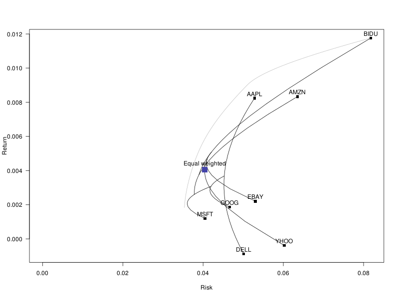
The mean-variance portfolios maximize the risk-adjusted expected returns of the portfolio.
Expected return - lambda * Risk
The risk-adjustment depends on the risk aversion of the investor (informally, this corresponds to lambda, in the formula). As a measure of risk, we can use the variance of the portfolio returns, but there are many other choices.
library(quadprog)
# solve.QP(Dmat, dvec, Amat, bvec, meq=0)
#   Find w
#   to maximize  d' w - 1/2 w' D w
#   such that    A' q >= b   (the first meq constraints are equalities)

# No constraints
n <- length(mu)
r <- solve.QP(V, mu, matrix(nr=n,nc=0), c())
round( r$solution, 2 ) # The leverage is too high

# The weights should sum up to 1
A <- matrix( rep(1,n), nr=n )
b <- 1
r <- solve.QP(V, mu, A, b, meq=1) # The first constraint is an equality
sum(r$solution) # 1
round( r$solution, 2 ) # The leverage is still too high

# Long-only portfolio: ask that the weights be positive
A <- cbind( # Each column is a constraint
  matrix( rep(1,n), nr=n ),
  diag(n)
)
b <- c(1, rep(0,n))
r <- solve.QP(V, mu, A, b, meq=1)
sum(r$solution) # 1
round(r$solution, 2 ) # Very concentrated...

plot_portfolio( r$solution, "mean variance" )

# More risk-averse investor
plot_portfolio( solve.QP(10*V, mu, A, b, meq=1)$solution, "mean variance" )
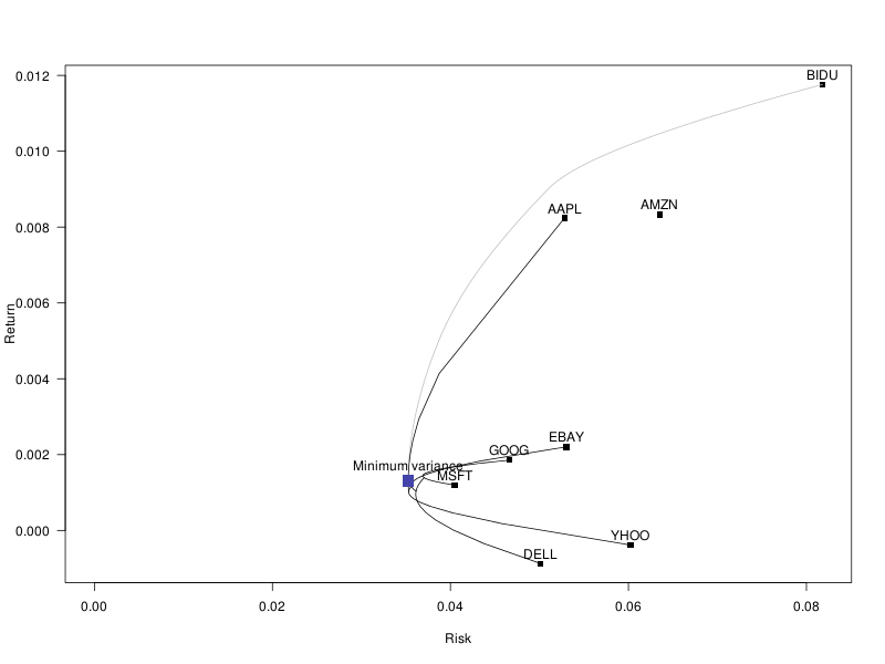
Instead of looking at the risk-adjusted returns, we can just look at the risk -- it is much easier to predict future risk than future returns.
# Minimum variance portfolio
r <- solve.QP(V, 0*mu, A, b, meq=1)
w_minimum_variance <- r$solution
plot_portfolio( r$solution, "Minimum variance" )
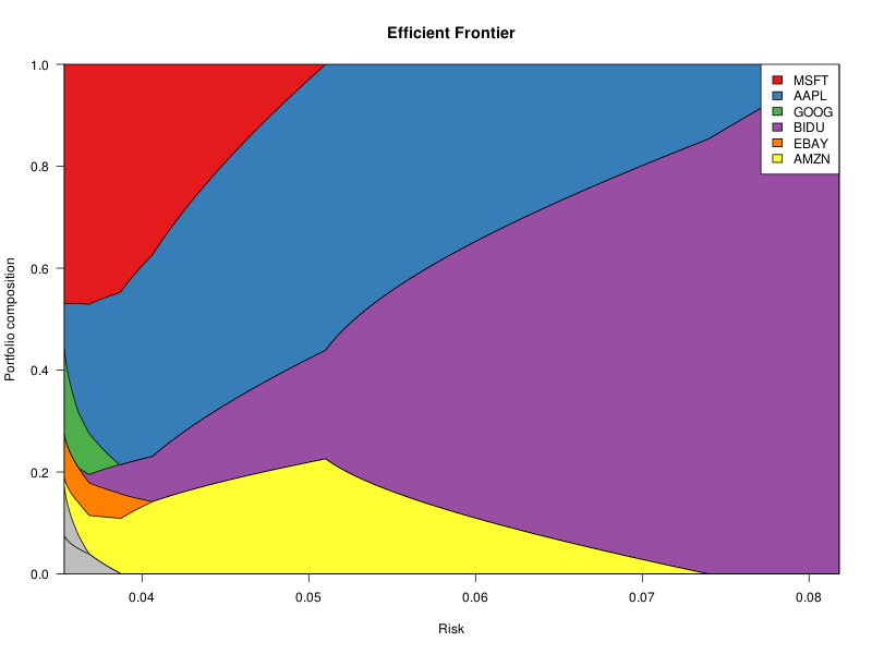
There are several ways of identifying the portfolios on the efficient frontier:
Minimize w' V w   such that w' mu  = mu0
Minimize w' V w   such that w' mu >= mu0
Maximize w' mu    such that w' V w  = v0
Maximize w' mu    such that w' V w <= v0
Maximize w' mu - lambda w' V w
They correspond to minimizing the risk for a fixed target expected return, maximizing the returns for a fixed risk budget, and maximizing the risk-adjusted returns.
Unfortunately, as you add more constraints (fully invested, no short sales, weight limits for each sector, weight limits for each asset, limit on the number of assets, lot sizes, etc.), the shape of the feasible region changes and need not remain convex: those problems are no longer guaranteed to be equivalent.
# Efficient frontier, long-only, no other constraints
r <- solve.QP(V, 0*mu, A, b, meq=1)
frontier <- plot_portfolio( r$solution, "Minimum variance" )
risk <- sqrt(colSums( frontier * (V %*% frontier) ))
cumplot <- function(x, y) {
  if(missing(y)) {
    y <- x
    x <- index(x)
  }
  # Change the order so that the most important elements be first
  i <- order(apply(y, 1, mean, na.rm=TRUE), decreasing=TRUE)
  j <- order(apply(y, 1, max,  na.rm=TRUE), decreasing=TRUE)
  n <- length(i)
  i <- c(
    i[1:min(3,n)],
    j[1:min(3,n)],
    i
  )
  i <- i[ !duplicated(i) ]
  y <- y[rev(i),]
  # Cumulated sum
  yc <- t(apply(y,2,cumsum))
  # Plot
  require(RColorBrewer)
  palette <- brewer.pal(6, "Set1")
  palette <- rev(c(palette, rep("grey", n))[1:n])
  matplot(
    x, yc,
    las=1, type="n", xlab="", ylab="",
    xaxs="i", yaxs="i"
  )
  m <- dim(y)[2]
  for(i in n:1) {
    polygon(c(x[1],x,x[m]), c(0,yc[,i],0), col=palette[i])
  }
  legend("topright",
    rev(rownames(y)) [1:min(6,dim(y)[1])],
    fill=rev(palette)[1:min(6,dim(y)[1])],
    bg="white"
  )
}
cumplot(risk, frontier)
title(
  xlab="Risk",
  ylab="Portfolio composition",
  main="Efficient Frontier"
)
# If we add cardinality constraints, the feasible region
# becomes non-convex.
# There are actually big holes in the feasible region,
# very visible if you ask for just 2 assets.
n <- 1e4
k <- 2
w <- matrix( rexp(k*n), nc=k )
w <- t(apply( w, 1, function(u) {
  x <- 0*mu
  x[sample(seq_along(mu),k)] <- u
  x/sum(u)
} ))
plot_random_portfolios(w, "Non-convex feasible region")

# The efficient frontier is not connected
x <- data.frame(
  risk   = apply(w, 1, function(u) sqrt(t(u) %*% V %*% u) ),
  return = w %*% mu
)
library(sqldf)
# Skyline query (there are faster algorithms, but this one is more readable)
y <- sqldf("
  SELECT *
  FROM x AS A
  WHERE NOT EXISTS(
    SELECT * FROM x AS B
    WHERE B.return >  A.return AND B.risk <= A.risk
    OR    B.return >= A.return AND B.risk <  A.risk
  )
")
plot_assets()
points(x, pch=".")
points(y, pch=15, col="navy")
legend("topleft", "Efficient frontier", col="navy", lty=1, lwd=5, bg="white")
title(main="Non-connected efficient frontier")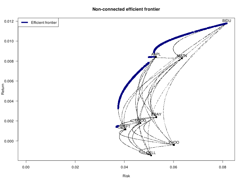
A very naive way of finding a (near-)optimal portfolio, for an arbitrary objective function, would be to take many portfolios at random, and keep the best one.
At first, it seems a very bad idea: we are apparently just sampling from portfolios around the equal-weighted portfolio.
# Incorrectly biased random portfolios
n <- 1e4
w <- matrix( runif(n*length(mu)), nc=length(mu) )
w <- t(apply(w, 1, function(u) u / sum(u)))
plot_random_portfolios <- function(w, title, V=V0, mu=mu0) {
  plot_assets(V=V, mu=mu)
  plot_efficient_frontier(V=V, mu=mu)
  points(
    apply(w, 1, function(u) sqrt(t(u) %*% V %*% u) ),
    w %*% mu,
    pch=16, col="#44444422"
  )
  par(new=TRUE)
  plot_assets(V=V,mu=mu)
  mtext(title, font=2, line=1 )
}
plot_random_portfolios(w, "Random portfolios, the wrong way")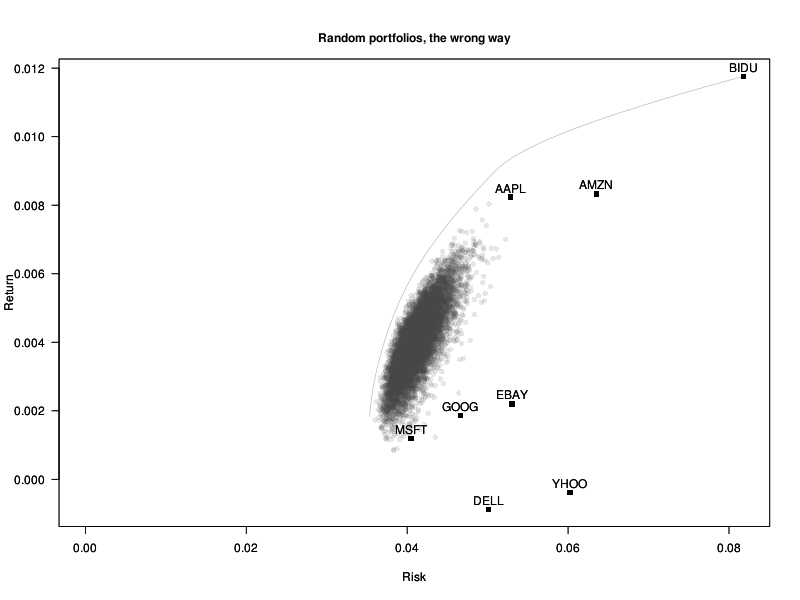
But there are many things we are doing wrong.
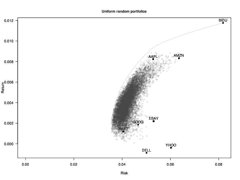
First, if we take uniformly distributed numbers and divide them by their sum, we do not have uniformly distributed numbers in the simplex [sum(w)=1]: there is a bias towards the center of the simplex. It disappears if we use an exponential distribution instead: we are now much closer to the efficient frontier.
# Uniform random portfolios
w <- matrix( rexp(n*length(mu),1), nc=length(mu) )
w <- t(apply(w, 1, function(u) u / sum(u)))
plot_random_portfolios(w, "Uniform random portfolios")
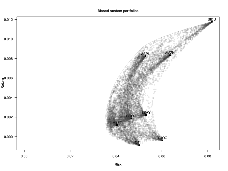
We do not really want to sample uniformly from the simplex: optimal portfolios tend to be somewhere on the boundary. Taking some power of the weights will bias the data towards the vertices and the edges. (The value is a bit too high, so that we can see on the plot what actually happens.)
# Biased random portfolios
# For more details:
#   Portfolio Optimization for VAR, CVaR, Omega and Utility with General Return Distributions
#   W.T. Shaw
#   http://papers.ssrn.com/sol3/papers.cfm?abstract_id=1856476
w <- matrix( rexp(n*length(mu),1), nc=length(mu) )
w <- w^4
w <- t(apply(w, 1, function(u) u / sum(u)))
plot_random_portfolios(w, "Biased random portfolios")
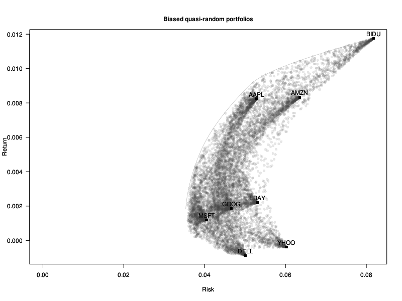
We could improve things further by using low-discrepancy sequences.
# Biased quasi-random portfolios
library(randtoolbox)
w <- sobol(n,length(mu))
w <- -log(w)
w <- w^4
w_random_portfolios <-
w <- t(apply(w, 1, function(u) u / sum(u)))
plot_random_portfolios(w, "Biased quasi-random portfolios")
With more stocks, you may want to increase the exponent, but not too much, otherwise most portfolios are concentrated on a single stock.
op <- par(mfrow=c(3,3),mar=c(0,0,0,0))
for(i in c(1,2,3, 5,10,15, 20,35,50)) {
  w <- matrix( rexp(n*length(mu1),1), nc=length(mu1) )
  w <- w^i
  w <- t(apply(w, 1, function(u) u / sum(u)))
  plot(
    apply(w, 1, function(u) sqrt(t(u) %*% V1 %*% u) ),
    w %*% mu1,
    pch=16, col="#44444422",
    axes = FALSE, xlab="", ylab="", main="",
    xlim=c(0,.14), ylim=c(-.01,.004),
  )
  box()
}
par(op)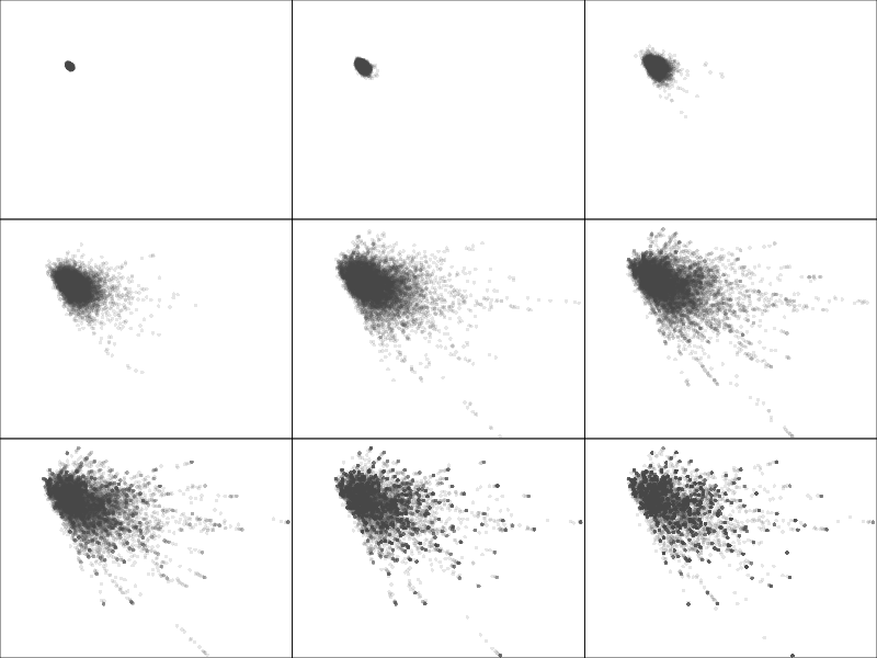
The unconstrained long-short portfolio has an excessive leverage. We can control the leverage in the same way we implemented quantile regression: write the portfolio weights as w[i] = a[i] - b[i], with a and b positive.
n <- length(mu)
A <- cbind( # Each column is a constraint
  matrix( c(rep(1,n), rep(0,n)), nr=2*n ),
  matrix( c(rep(0,n), rep(1,n)), nr=2*n ),
  diag(2*n)
)
b <- c(1.3, .3, rep(0,2*n))  # 130% long, 30% short
VV <- rbind( cbind(V,-V), cbind(-V,V) )
VV <- kronecker( matrix(c(1,-1,-1,1), 2), V )
# solve.QP wants a positive definite matrix:
# truncate the eigenvalues, and hope that it has no effect
# on the stability of the algorithm (I am dubious...).
e <- eigen(VV)
VV <- e$vectors %*% diag(pmax(1e-6,e$values)) %*% t(e$vectors)
r <- solve.QP( 5 * VV, c(mu,-mu), A, b, meq=2)
w <- matrix(r$solution, nc=2)
w <- w[,1] - w[,2]
sum(w); sum(w[w>0]); sum(w[w<0])
plot_portfolio( w, "130/30" )

# Add the 130/30 efficient frontier
f <- function(u) {
  r <- solve.QP( u * VV, c(mu,-mu), A, b, meq=2)
  w <- matrix(r$solution, nc=2)
  w <- w[,1] - w[,2]
  c(sqrt(t(w) %*% V %*% w), t(w) %*% mu)
}
lines( t(sapply( exp(.3*(4:20)), f)) )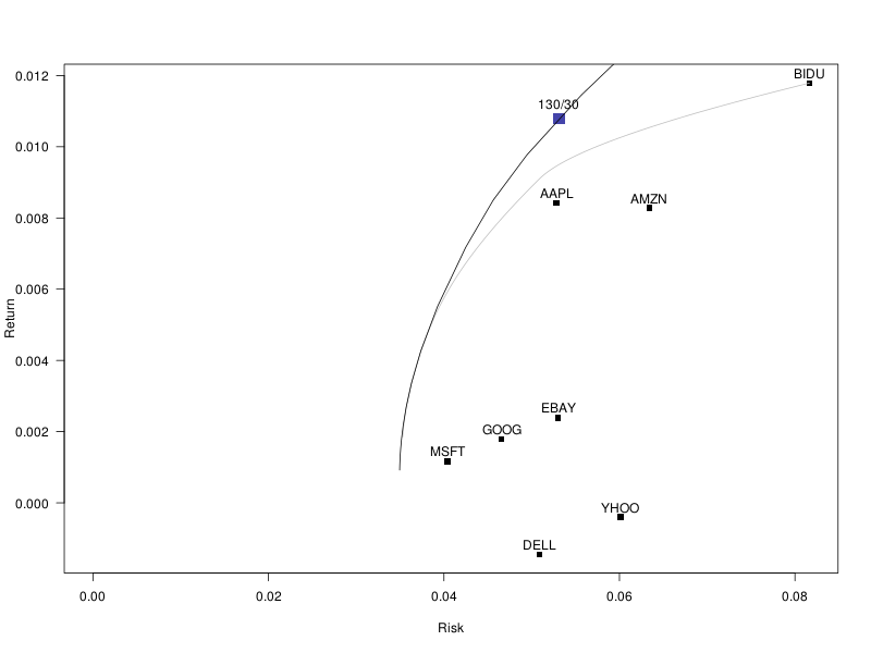
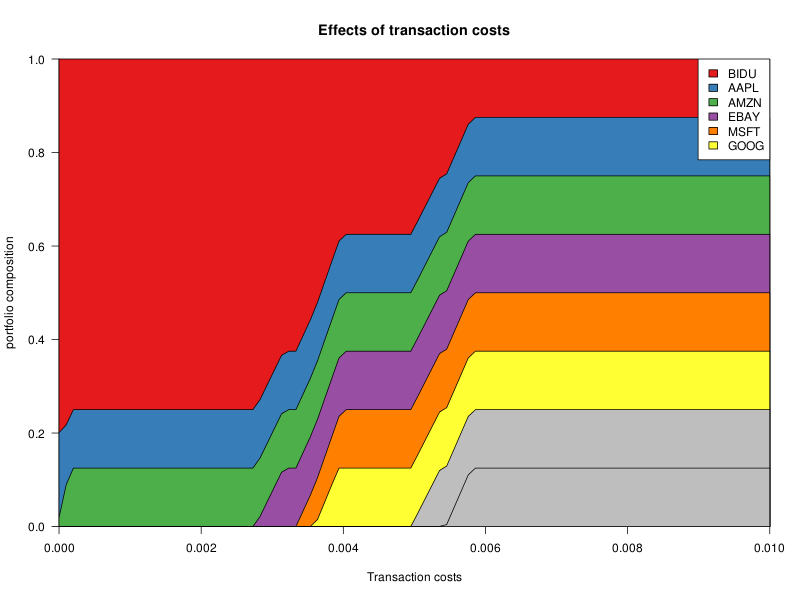
Transaction costs can be added as a penalty to the objective function. The easiest to solve is an L2 penalty: the problem remains quadratic.
Maximize w' mu - lambda w' V w - (w-w0)' Cost (w-w0)
i.e.,    w' ( mu + 2 Cost w0 ) - w' ( lambda V + Cost ) w
But a linear penalty is more realistic.
Maximize w' mu - lambda w' V w - abs(w-w0)' Cost
We can get rid of the absolute value as usual, by writing its argument as a difference of two numbers.
Find        w, a, b
to maximize w' mu - (a+b)' Cost - lambda w' V w
such that   a, b >= 0
            w = w0 + a - b
In code:
f <- function(cost, w0, mu=mu0, V=V0) {
  n <- length(mu)
  # The quadprog package only deals with strictly convex problems,
  # i.e., positive definite quadratic forms.
  # Since the variables we have added to remove the absolute value
  # do not appear in the quadratic term, our matrix is only
  # positive semi-definite.
  # Tweak the matrix to make it positive definite
  # (of course, you should not do that).
  VV <- 1e-8 * diag(n)
  VV <- rbind(
    cbind(V,   0*V, 0*V),
    cbind(0*V,  VV, 0*V),
    cbind(0*V, 0*V,  VV)
  )
  r <- solve.QP(
    VV,
    c(mu, -cost, -cost),
    cbind(
      c( rep(1,n), rep(0,2*n) ),        # w' 1 = 1
      rbind(diag(n),-diag(n),diag(n)),  # w - w0 = a - b
      diag(3*n)                         # w, a, b >= 0
    ),
    c(1, w0, rep(0,3*n)),
    meq=1+n
  )
  r$solution[1:n]
}
n <- length(mu0)
w0 <- rep(1/n,n)  # The current portfolio is equal-weighted
cost <- seq(0,.01,length=100)
y <- sapply( cost, function(u) f(cost=0*mu+u, w0=w0) )
rownames(y) <- names(mu)
cumplot(cost, y)
title(
  xlab="Transaction costs",
  ylab="portfolio composition",
  main="Effects of transaction costs"
)
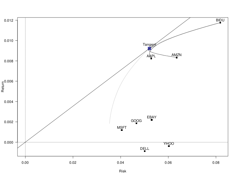
We could first compute all the portfolios on the efficient frontier, and then find the tangent one among them. But that is a lot of computations if you only want one portfolio (all the more so when there are many assets).
Alternatively, we can use a non-linear optimizer (at first sight, maximizing the Sharpe ratio does not look like a quadratic problem).
library(Rsolnp)
r <- solnp(
  rep(1/length(mu), length(mu)),
  function(w) - t(w) %*% mu / sqrt( t(w) %*% V %*% w ),
  eqfun = function(w) sum(w),
  eqB   = 1,
  LB = rep(0, length(mu))
)
plot_portfolio( r$pars, "Tangent" )

# Let us try with another non-linear optimizer
library(alabama)
r <- constrOptim.nl(
  rep(1/length(mu), length(mu)),
  function(w) - t(w) %*% mu / sqrt( t(w) %*% V %*% w ),
  hin = function(w) w,
  heq = function(w) sum(w) - 1
)
plot_portfolio( r$par, "Tangent" )
abline(0, t(r$par) %*% mu / sqrt( t(r$par) %*% V %*% r$par ) )
abline(h=0, v=0, lty=3)
But it is not a convex problem: there is no guarantee that the solution we get is a global maximum.
# The equal-weighted portfolio is a saddle point
library(numDeriv)
f <- function(w) - t(w) %*% mu / sqrt( t(w) %*% V %*% w )
h <- hessian(f, rep(1/length(mu), length(mu)))
round( eigen(h)$values, 2 )
# 1.04  0.18  0.13  0.10  0.09  0.07  0.06 -0.60
It turns out that the problem of finding the tangent portfolio can be reformulated as a quadratic problem, as follows. The tangent portfolio is also the maximum Sharpe ratio portfolio, where the Sharpe ratio is w' mu / sqrt(w' V w), among fully-invested portfolios (the weights should sum up to 1). Let us remove the constraint that the weights sum up to 1. There is no longer a unique solution to the problem: since the Share ratio in unchanged when we multiply the weights by a non-zero number (it is homogeneous of degree 0), the maximum Sharpe ratio portfolios form a line -- once we know one portfolio, we can obtain the others by multiplying it by a scalar. To have a single solution, we can impose a condition on the weights. For instance, we can ask that the numerator of the Share ratio be 1. We then have to maximize 1/sqrt( w' V w ), i.e., to minimize w' V w: that is a quadratic problem.
# No short-selling constraint
r <- solve.QP( V, 0*mu, matrix(mu), 1, meq=0 )
w <- r$solution / sum(r$solution)

# Long-only
r <- solve.QP( V, 0*mu,
  cbind(matrix(mu),diag(length(mu))),
  c(1,rep(0,length(mu))),
  meq=0
)
w <- r$solution / sum(r$solution)

plot_portfolio( w, "Tangent" )
abline(0, t(w) %*% mu / sqrt( t(w) %*% V %*% w ) )
abline(h=0, v=0, lty=3)
The conditional value at risk (CVaR), also called expected shortfall (ES), is the expected loss, given that the loss is beyond some threshold.
E[ - Returns | - Returns > Threshold ]
The threshold is usually some quantile of the distribution of returns, e.g., the 5% quantile, or the 1% quantile.
We can use the expected shortfall as a measure of risk.
If we knew the distribution of the returns, that would simply be a non-linear optimization problem.
# CVaR optimization, assuming gaussian returns
library(Rsolnp)
alpha <- 0.01
r <- solnp(
  rep(1/length(mu), length(mu)),
  function(w) - qnorm(alpha, t(w) %*% mu, sqrt( t(w) %*% V %*% w ) ),
  eqfun = function(w) sum(w),
  eqB   = 1 ,
  LB = rep(0, length(mu))
)
# Since the CVaR is a monotonic function
# of the variance, we get, unsurprisingly,
# the minimum variance portfolio.
plot_portfolio( r$pars, "CVaR 1%" )
However, returns are not gaussian.
x <- as.vector(as.matrix(d[-1,-1]))
x <- (x-mean(x))/sd(x)
plot(density(x),
  lwd=3, col="navy", las=1, log="y", ylim=c(1e-4,1),
  main="Daily stock returns are not Gaussian"
)
curve( dnorm(x), lwd=3, lty=2, add=TRUE )
legend("topleft",
  c("Return density", "Gaussian density"),
  col=c("navy","black"),
  lwd=3,
  lty=c(1,2)
)

qqnorm(x)
qqline(x)
(We could use other parametric distributions.)
Instead of a parametric distribution, we can use the empirical distribution of the returns.
First, we need to express the (sample) expected shortfall as an optimization problem. It is the minimum, over u, of
u + 1/alpha * mean( pmax(-x-u,0) )
In R:
# Expected shortfall
# The average loss (opposite of the returns),
# given that the loss exceeds the 10% quantile
n <- 1e3
x <- sort(rnorm(n))
alpha <- .1
f <- function(u) u + 1/alpha * mean( pmax(-x-u,0) )
min( sapply(seq(-5,5,by=.01), f) )
mean(x[ (1:n) <= n*alpha ])

CVaR <- function(x, alpha) {
  u <- seq(-5,5,length=1e3)
  y <- sapply(u, function(u) u + mean(pmax(0,-x-u))/alpha)
  i <- which.min(y)
  result <- y[i]
  attr(result, "u") <- u[i]
  result
}
alpha <- .05
CVaR( rnorm(1e4), alpha )
-qnorm(alpha)  # u is the quantile
- exp( - qnorm(alpha)^2 / 2 ) / sqrt( 2 * pi ) / alpha
The optimization problem becomes a bit messy (if you make a mistake somewhere, e.g., with the sign of the slack variables, the bug is extremely time-consuming to track down)...
Find        u, w, a, b
To minimize -w' mu + lambda ( u + 1/alpha * 1/n * b' 1 )
Such that   w' 1 = 1
            w, a, b >= 0
            a - b = X w + u 1
In R:
lambda <- .5                         # Risk aversion
alpha  <- .05                        # The quantile we are interested in
X <- d[apply( !is.na(d), 1, all ),]  # Scenarios
X <- as.matrix(X[,-1])
n <- dim(X)[1]
# Objective
obj <- c(lambda, -mu, rep(0,n), rep(lambda/alpha/n, n))
# Constraints, one per line
A1 <- t(c(0, rep(1, length(mu)), rep(0,n), rep(0,n) ))
b1 <- 1
d1 <- "=="
A2 <- cbind(0, diag(2*n+length(mu)))
b2 <- rep(0, 2*n+length(mu))
d2 <- rep(">=", length(b2))
A3 <- cbind(1, X, -diag(n), diag(n))
b3 <- rep(0,n)
d3 <- rep("==",length(b3))
# Solve the problem
library(lpSolve)
r <- lp("min",
  obj,
  rbind(A1, A2, A3),
  c(d1, d2, d3),   # Be careful: if you get the direction vector wrong, there is no error message...
  c(b1, b2, b3)
)
stopifnot( r$status == 0 )
w0 <- r$solution[-1][1:length(mu)]
t(r$solution) %*% c(1, 0*mu, rep(0,n), rep(1/alpha/n, n))
plot_portfolio( w0, "CVaR 5%" )

# Same result with another optimizer
library(Rglpk)
r <- Rglpk_solve_LP(
  obj,
  rbind(A1, A2, A3),
  c(d1, d2, d3),
  c(b1, b2, b3),
  bounds = list( lower=list( ind=1, val=-Inf ),
                 upper=list( ind=1, val=+Inf ) )
)
round( cbind(w0, r$solution[-1][1:length(mu)]), 3 )
To ensure that we are indeed minimizing the expected shortfall, let us compare with a more direct optimization.
ES <- function(x, alpha) -mean(x[x <= quantile(x,alpha)])
f <- function(w) - t(w) %*% mu + lambda * ES(X %*% w, alpha)
f(w0)

r <- solnp(
  rep(1/length(mu), length(mu)),
  f,
  eqfun = function(w) sum(w),
  eqB   = 1 ,
  LB = rep(0, length(mu))
)
round( 100 * cbind(w, r$pars) )
f(w0); f(r$pars)  # Almost identical

library(DEoptim)
r <- DEoptim( function(u) f(u/sum(u)), lower=0*mu, upper=0*mu+1 )
w <- r$optim$bestmem
w <- w / sum(w)
f(w); f(w0) # Almost identical
In a similar way, we could add a constraint on the CVaR.
The value at risk (VaR) is just a quantile of the distribution of returns -- but it is expressed as a loss, so the sign is different.
It can be expressed as follows,
VaR = - Argmin_\tau \sum_i (1-\alpha) (x_i-\tau)_- + \alpha (x_i-\tau)_+
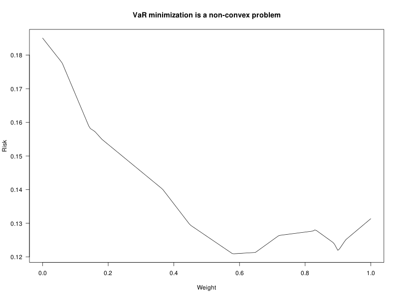
= Min( \tau : 1/n * \sum_i 1_{-\tau \leq x_i} > \alpha ).Since this is a minimum, it can be used in the objective function of an optimization problem, as we did for the CVaR. Unfortunately, the indicator functions (which can be encoded with binary variables) make the optimization problem (non-convex and) rather difficult to solve.
x <- seq(0,1,length=200)
f <- function(u) quantile(
  as.matrix(d[-1,c(6,7)]) %*% c(u,1-u),
  c(.01,.05,.1,.2)
)
y <- -t(sapply(x,f))
matplot(
  x, y[,1],
  las=1, type="l", lty=1,
  ylab="Risk", xlab="Weight",
  main="VaR minimization is a non-convex problem"
)
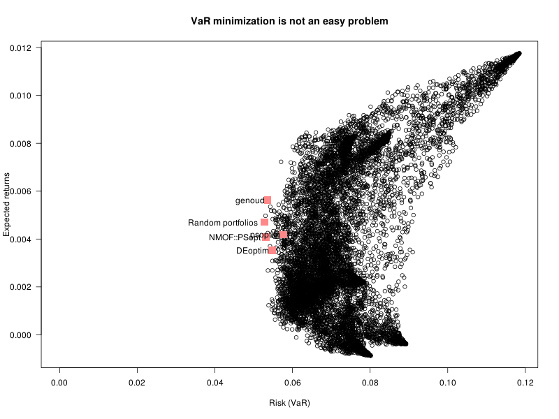
We can use some robust optimizer, e.g., DEoptim.
alpha <- .05
f <- function(w) {
  # Penalty for negative weights and weights that do not sum up to 1
  penalty <- - sum( w[ w < 0 ] ) + abs( sum(w) - 1 )
  w <- abs(w) / sum(abs(w))
  - quantile( X %*% w, alpha ) + penalty
}

# Random portfolios
risk <- apply( w_random_portfolios, 1, f )
i <- which.min(risk)
w0 <- w_random_portfolios[i,]
risk[i]

library(DEoptim)
r1 <- DEoptim( f, lower=0*mu, upper=0*mu+1 )
w1 <- r1$optim$bestmem

library(rgenoud)
r2 <- genoud(f, nvars=length(mu))  # Slow. Often fails.
w2 <- r2$par

library(pso)
n <- length(mu)
r3 <- psoptim(runif(n), f, lower=0, upper=1)
w3 <- r3$par

library(NMOF)
r4 <- PSopt(f, list(min=rep(0,length(mu)), max=rep(1,length(mu))))
w4 <- r4$xbest

library(NMOF)
r5 <- TAopt(f, list(
  x0 = runif(length(mu)),
  neighbour = function(u) u + .05*rnorm(length(u))
))
w5 <- r5$xbest

plot(
  risk, w_random_portfolios %*% mu,
  las=1,
  xlim=range(c(0,risk)),
  xlab="Risk (VaR)", ylab="Expected returns",
  main="VaR minimization is not an easy problem"
)
x <- rbind(
  w0,w1,w2,w3,w4,w5
  # With out-of-sample data, we would also compare
  # with other reference portfolios: they solve other
  # problems but could end up being better (though biased)
  # estimators of the minimum VaR portfolio.
  #w_minimum_variance,
  #rep(1/length(mu), length(mu))
)
points(
  apply(x, 1, f), x %*% mu,
  pch=15, col="#FF8888", cex=2
)
text(apply(x, 1, f), x %*% mu,
  labels=c(
    "Random portfolios",
    "DEoptim", "genoud", "psoptim", "NMOF::PSopt", "NMOF::TAopt"
    #"Minimum Variance", "Equal-weighted"
  ),
  adj=c(1.1,.5)
)
Adding the constraint that some of the variables are binary, i.e., can only take two values, 0 or 1, makes the problem even more combinatorial. If there are n such binary variables, we can solve the 2^n problems corresponding to all their possibles values. That is too much, of course, but we can reduce the number of problems to solve by arranging them into a tree, finding a bound on the value of each subtree, and pruning all subtrees as follows. The root of the tree corresponds to the unconstrained problem: the binary variables are only constrained to be in [0,1], but they do not have to be integers. There are two children nodes, each adding a constraint on the first binary variable: it is either 0 or 1 (the other variables remain in [0,1]). The next layer of the tree (4 nodes) adds constraints on the second variable, and so on. We are looking for the leaf with the best solution. Since the nodes have less stringent constraints than the leaves, their solution is better, but never worse, that the leaves below them: if the value of a node is worse than the best leaf solution found so far, there is no need to explore the subtree, and it can be pruned.
In the following example, we consider the problem of finding the minimum variance, long-only portfolio, with at most 5 assets.
The problem can be written as
Find      w, b (vectors of length n)
Minimize  - w' V w
Such that w' 1 = 1
          b' 1 = 5
          0 <= w <= b
          b binary
Let us first write functions to add constraints and solve the problem (so that the code can be reused with other solvers).
n <- length(mu)
problem <- list(
  Dmat = rbind( cbind(V,0*V), cbind(0*V,1e-8*diag(n)) ), # solve.QP only accepts positive definite matrices
  dvec = c(0*mu,0*mu),
  Amat = cbind(
    c(1+0*mu,0*mu),            # w' 1 = 1
    c(0*mu,1+0*mu),            # b' 1 = 5
    rbind(diag(n),0*diag(n)),  # w >= 0
    rbind(-diag(n), diag(n)),  # b - w >= 0
    rbind(0*diag(n),diag(n)),  # b >= 0
    rbind(0*diag(n),-diag(n))  # b <= 1
  ),
  bvec = c(1,5,rep(0,n),rep(0,n), rep(0,n), rep(-1,n)),
  meq = 2
)
add_constraint <- function( problem, i, value ) {
  Amat <- cbind( 0*problem$dvec, problem$Amat )
  Amat[i,1] <- 1
  bvec <- c(value, problem$bvec)
  meq  <- problem$meq + 1

  result <- problem
  result$Amat <- Amat
  result$bvec <- bvec
  result$meq  <- meq
  result
}
solve <- function(problem) {
  r <- NULL
  try(
    r <- solve.QP(
      problem$Dmat, problem$dvec,
      problem$Amat, problem$bvec,
      problem$meq
    ),
    silent = TRUE
  )
  # Logging: indicate which variables are fixed
  x <- rep(".", length(problem$dvec))
  j <- apply(problem$Amat != 0, 2, sum) == 1  # Constraints of the form x[i] =,>=,<= a
  j <- (1:problem$meq)[ j[1:problem$meq] ]    # Equalities
  if(length(j) > 0 ) {
    i <- apply(problem$Amat[,j,drop=FALSE]!=0, 2, which)
    x[i] <- "*"
  }
  cat(paste(x,collapse=""))
  if( !is.null(r) ) {
    cat(" ", r$value, "\n")
    list(
      solution = r$solution,
      value    = r$value
    )
  } else {
    cat("  Inf\n")
    list(value=Inf)
  }
}
solve(problem)
solve( add_constraint(problem, n+1, 1) )
solve( add_constraint(problem, n+1, 0) )

solveb <- function(problem, binary_variables, best=list(value=Inf)) {
  # Leaf
  if(length(binary_variables) == 0) {
    return( solve(problem) )
  }
  # Should we prune the subtree?
  r <- solve(problem)
  if( r$value >= best$value ) {
    cat("Pruning 2^", length(binary_variables), " leaves\n", sep="")
    return( best )
  }
  # Explore the subtree
  i <- binary_variables[1]   # Variable to constrain
  v <- sample(0:1,1)         # Should we first check 0 and the 1, or the opposite?
  p0 <- add_constraint(problem, i, v)
  p1 <- add_constraint(problem, i, 1-v)
  r <- solveb(p0, binary_variables[-1], best)
  if(r$value < best$value)
    best <- r
  r <- solveb(p1, binary_variables[-1], best)
  if(r$value < best$value)
    best <- r
  best
}

r <- solveb(problem, n+(1:n))
round(r$solution,2)[1:n]

plot_portfolio( r$solution[1:n], "Minimum variance, at most 5 assets" )The same idea can be used to handle integrality constants: at each node, we split the tree into 3 subtrees, corresponding to the constraints x[i]=v (where v is some integer value, e.g., the integer closest to the solution of the unconstrained problem), x[i] >= v+1 and x[i] <= v-1. The tree can be much larger than in the binary case: only when we add an equality constraint does the number of variables to decide on decrease. (In most cases, the x[i] are bounded, so that the tree is finite.)
The algorithm can be improved: you can split the nodes in 2 rather than 3, you can carefully choose the variable to split on, you can use better heuristics to find a good upper bound on the minimum, you can add constraints to shrink the set of feasible solutions ("branch-and-cut).
n <- length(mu)
problem <- list(
  Dmat = V,
  dvec = 0*mu,
  # The weights are in percents and we want a whole number of percents.
  # In a real-world situation, this would be the number of shares
  # (you cannot buy half a share) of the number of lots
  # (some shares can only be bought by lots of 100 or 1000 shares).
  Amat = cbind(
    rep(1,n),      # w' 1 = 100
    diag(n)        # w >= 0
  ),
  bvec = c(100,rep(0,n)),
  meq = 1
)

add_constraint <- function( problem, i, value, side ) {
  if(side == 0) {
    # side = 0: add an equality constraint
    Amat <- cbind( 0*problem$dvec, problem$Amat )
    Amat[i,1] <- 1
    bvec <- c(value, problem$bvec)
    meq  <- problem$meq + 1
  } else {
    # side = +1 or -1: add an inequality x[i] >= v or x[i] <= v
    Amat <- cbind( problem$Amat, 0*problem$dvec )
    Amat[i,dim(Amat)[2]] <- side
    bvec <- c(problem$bvec, side * value)
    meq  <- problem$meq
  }

  result <- problem
  result$Amat <- Amat
  result$bvec <- bvec
  result$meq  <- meq
  result
}

solve(problem)
solve(add_constraint(problem, 1, 5,  0))
solve(add_constraint(problem, 1, 5,  1))
solve(add_constraint(problem, 1, 5, -1))

solvei <- function(problem, integral_variables, best=list(value=Inf)) {
  # Leaf
  if(length(integral_variables) == 0) {
    return( solve(problem) )
  }
  # Should we prune the subtree?
  r <- solve(problem)
  if( r$value >= best$value ) {
    cat("Pruning ", length(integral_variables), " variables\n", sep="")
    return( best )
  }
  # Explore the 3 subtrees
  i <- integral_variables[1]   # Variable to constrain
  v <- r$solution[i]
  p0 <- add_constraint(problem, i, round(v),   side=0)
  p1 <- add_constraint(problem, i, round(v)+1, side=1)
  p2 <- add_constraint(problem, i, round(v)-1, side=-1)

  r <- solvei(p0, integral_variables[-1], best)
  if(r$value < best$value)
    best <- r

  r <- solvei(p1, sample(integral_variables), best)
  if(r$value < best$value)
    best <- r

  r <- solvei(p2, sample(integral_variables), best)
  if(r$value < best$value)
    best <- r

  best
}

r <- solvei(problem, 1:n)  # Very slow...
round(r$solution,2)

# Compare with the unconstrained solution
r0 <- solve.QP(V, 0*mu, cbind(rep(1,n),diag(n)), c(1,rep(0,n)))
round(rbind( r$solution, 100*r0$solution ), 2)The risk of a portfolio,
Risk(w) = sqrt( w' V w )
is homogeneous of degree 1, and can therefore be decomposed as
Risk(w) = \sum_i w_i  d Risk / d w_i
        = \sum_i w_i MCTR_i(w)
where the marginal contribution to risk (MCTR) of asset i can be computed as
MCTR_i(w) = V[i,] w / Risk.
Let us check on an example:
risk <- function(w, V=V0) sqrt( t(w) %*% V %*% w )
library(numDeriv)
w <- rep(1/length(mu), length(mu))
risk(w)
mctr <- grad(risk, w)
sum( w * mctr )
mctr <- drop(V %*% w) / sqrt(t(w) %*% V %*% w)
sum( w * mctr )
It is easy to find portfolios with equal marginal contribution to risk. It is not really an optimization problem, but just a system of equations to solve. If r is the vector of desired marginal contributions to risk (up to a multiplicative constant), we want w (and lambda) such that
V w / sqrt( w' V w ) = lambda r
sqrt( w' V w ) = target risk
which gives
w = target risk / sqrt( r' V^-1 r ) V^-1 r.
In code:
risk <- function(w) sqrt(t(w) %*% V %*% w)
mctr <- function(w, V=V0) drop(V %*% w) / risk(w)
n  <- length(mu)
w0 <- rep(1/n,n) # Same risk as the equal-weighted portfolio
r  <- rep(1/n,n) # Equal marginal contributions to risk
w <- risk(w0) / sqrt( t(r) %*% solve(V, r) ) * solve(V, r)
mctr(w)  # All equal
plot_portfolio( w, "Equal MCTR" )
In a risk parity portfolio, the assets have the same contribution to risk (the contribution to risk is w*MCTR). They are a special case of risk budgeting portfolios, where the contribution to risk of each asset is imposed. It is still a system of equations to solve, but it is not linear: if r_i is the desired contribution to risk of asset i, we want to find w so that
w_i V[i,] w / Risk = r_i
where the risk is the sum of the contributions to risk. This can be written as
w . V w = sum(r) r
where . is the elementwise product.
In matrix form:
diag( w (V w)' ) = (r' 1) r
(It is a quadratic equation: no easy solution.)
We can use a non-linear solver.
# Contribution to risk
library(Rsolnp)
negentropy <- function(p) { p <- p / sum(p); sum( p * log(p) ) }
r <- solnp(
  rep(1/length(mu), length(mu)),
  function(w) negentropy( w * mctr(w) ),
  eqfun = function(w) risk(w),                # Same total risk as the
  eqB   = risk(rep(1/length(mu),length(mu))), # equal-weighted portfolio.
  LB = rep(0, length(mu))
)
plot_portfolio( r$pars, "Equal contribution to risk" )
r$pars * mctr( r$pars )
# Risk-parity portfolios are leveraged.
# There is actually a single portfolio,
# leveraged to reach the target risk.
sum(r$pars)

# With prescribed risk contributions
relative_entropy <- function(p,q) { # KL divergence
  p <- p / sum(p)
  q <- q / sum(q)
  sum( p * log(p/q) )
}
b <- rep(1,n)
b[1:2] <- 2
r <- solnp(
  rep(1/length(mu), length(mu)),
  function(w) relative_entropy( w * mctr(w), b ),
  eqfun = function(w) risk(w),                # Same total risk as the
  eqB   = risk(rep(1/length(mu),length(mu))), # equal-weighted portfolio.
  LB = rep(0, length(mu))
)
plot_portfolio( r$pars, "Prescribed contributions to risk" )
r$pars * mctr( r$pars )
Since the problem is not convex, you may want to try other optimizers (e.g., DEoptim).
# The problem is not convex
f <- function(w) relative_entropy( w * mctr(w), b )
eigen( hessian(f, w0) )$values
We have presented the algorithms behind commonly-used optimization routines. They fall into three broad categories: gradient-like methods, that try to find a direction in which the objective function is better (with many variants, some eschewing the gradient (Nelder-Mead), some using a biased gradient (conjugate gradient), some using the hessian, some approximating the hessian (L-BGFS), some using the specific form of the objective function to simplify the computations (Gauss-Newton, Levenberg-Marquardt)); combinatorial methods, that explore on the frontier of the feasible set, from vertex to vertex (or from facet to facet), to improve the objective function (simplex, generalized reduced gradient); interior point methods, that regularize the Kuhn-Tucker conditions g * lambda = 0 into g * lambda = tau, and let the regularization parameter tau decrease.
We have presented some code to add binary or integral constraints to an arbitrary optimization problem; and code to allow us to enter optimization problems in a human-readable form.
We have given a few portfolio optimization examples: minimum variance, mean-variance, CVaR, VaR, prescribed contribution to risk, using a variety of optimization algorithms, including random portfolios.
We saw that, for real-world problems, different optimizers may give different results: it is safer to use several optimizers (some lack robustness, some lack speed, some are user-unfriendly and their use is therefore bug-prone), check that the constraints are satisfied (especially if you have to transform the problem by hand to give it to the optimizer) and compare with some base-line algorithm (e.g., random portfolios).
I focused on the algorithms, without stressing how careful one should be when using them in a financial context. You need to check if the purportedly optimal portfolios are indeed close to optimal, out-of-sample -- and you need to clearly define what you mean by "optimal". This will not only depend on the optimization problems, but also on the estimators of variance and returns used. You should check how sensitive those optimization problems are to their inputs. You should also carry out a complete backtest, to check how consistent the resulting portfolios are over time: is their out-of-sample performance independent of the market regime? do they generate an excessive turnover?
I did not mention the use of copulas, volatility models, (semi-)parametric estimators of VaR and CVaR, spectral risk measures, drawdown.
I intended to but did not mention second order cone programming and semi-definite programming, which generalize quadratic programming, and can be used for quadratic constraints and robust optimization (i.e., situations where you do not have a single number for the variances and expected returns, but intervals). There is an Rcsdp package, but the documentation is scarce (only one example), the error messages cryptic, and the licence non-standard.
posted at: 19:18 | path: /R | permanent link to this entry
