Before changing jobs and moving, a few months ago, I cleaned my desk and read through (some of) the piles of papers that were cluttering it. The interesting articles I stumbled upon covered some of the following topics.
- Which probability distribution should I use to model asset returns?
- Regression algorithms work fine when the variable to predict is observable, when it is known on the training sample -- what can you do if only its long-term effects are observed?
- Principal component analysis (PCA) is often used with time series but completely forgets the time structure and potential time dependencies: is it possible to have a "dynamic PCA"?
- How can Markowitcz's efficient frontier be generalized to other (several) measures of performance and risk?
- Can expected utility theory account for psychological biases such as the desire for negative expected gains if potential gains are very large (as in lotteries)?
- Options also occur in the real (non-financial) world and option pricing leads to a (not so) surprising conclusion on the (higher) value of free software.
(There were also a bunch of articles about copulas, maximum entropy estimators and graphical models, but that will be for next time.)
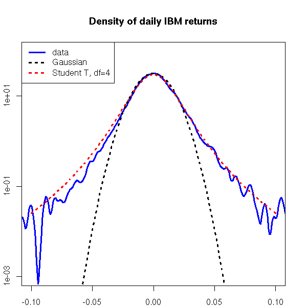
The gaussian distribution is supposed to be everywhere but, in finance, it does not faithfully describe log-returns.
Here is a small list of what people have tried to replace it:
- Student T distribution (my prefered, often with 4 degrees of freedom -- but check with your data, it depends on the frequency)
- Mixture of gaussians (a mixture of two gaussians with the same mean and different variances produces fat tails)
- GARCH models: they produce fat tails, even with gaussian innovations (a GARCH model can be seen as a continuous mixture of gaussians; equivalently, a mixture of gaussians can be seen as a discretization of a GARCH model, where the volatility only has two possible values and the time dimension has been discarded)
- Stable distributions: the central limit theorem can be generalized to distributions without a second moment; the limit distribution is then a stable distribution -- but except in a few cases, such as the gaussian and Cauchy distributions, they are not really amenable to computations
- Generalized hyperbolic distribution (yes, the definition is as complicated as it sounds)
- Johnson's $S_U$-normal distribution, a lon-linear transformation of a gaussian,
Y = sinh( lambda + theta X )
X ~ N(0,1)
The list could go on and on (in my notes, I have, without any definition: normal inverse gaussian, confluent U hypergeometric, generalized beta of the second kind, Pearson type IV, 4-moment maximum entropy, Edgeworth expansion, etc.), but when testing those fancy distributions against the Student T distribution, the latter still seems preferable.
The setup of a regression is very simple: you want to predict some variable (say, tomorrow's price of a stock) from other variables (the past movements of the stock price, the financial ratios of the company, etc.) and you have a training set (say, the past five years, for this and other companies) where both are observed.
But things are not always that simple: sometimes, the variable you are trying to predict is not observed -- if you are a shopkeeper trying to decide on the price of the items you are selling, the "best price", that will be sufficiently low to attract a large number of customers and sufficiently high to generate enough profit, is never observed -- you only know the price you chose. The 2-element (data/decision) regression framework can be replaced by the 3-element (data/decision/consequence) framework of reinforcement learning.
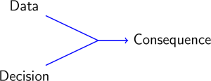
If we manage to predict the outcome (total revenue) of a decision (price) given the data (nature, cost, popularity, etc. of the item), i.e., if we manage to "learn" (think of neural networks) the arrow in the plot above, we can choose the decision (price) that will give the best outcome (highest revenue) given the current information.
The algorithms used in reinforcement learning are slightly more complicated: they add noise in the decision to take, in order to learn the (data,decision)-->outcome function on a wider set of decisions, i.e., they explore the space of decisions; they can also take into account delayed effects (in our shop example, higher or lower prices will not deter or attract clients immediately but progressively).
Reinforcement learning: a survey
L.P. Kaelbling et al.
Journal of artificial intelligence research (1996)
http://www.cs.cmu.edu/afs/cs/project/jair/pub/volume4/kaelbling96a.pdf
When estimating a large variance matrix (say, the variance of stock returns for a universe of a few thousand stocks), people often use a principal component analysis (PCA) or a factor analysis model: the variance matrix is assumed to be of the form
V = B v B' + D
where B is a rectangular matrix containing exposures to explanatory factors, v is the (smaller) variance matrix of those factors and D is a diagonal matrix containing the specific (i.e., not explained by the factors) variance -- in a PCA, there is no specific variance: D=0. Equivalently,
X_it = b_i f_t + u_it
where X_it is the return of stock i in period t, b_i are the exposures of stock i to the explanatory factors, f_t are the returns of the factors in period t and u_it is the residue.
But this assumes a complete time independence: the stock or factor returns in period t are independent of those in period t-1; this might be true for stock returns, but perhaps not for factor returns.
The dynamic factor model generalizes the factor model by allowing the factors to be auto-regressive (AR) time series.
An optimization problem (or an "optimization program" -- this terminology dates back to before the advent of computer programs) is the problem of maximizing (or minimizing) some function under a set of constraints. For instance, if you are a portfolio manager, your job is to "maximize the expected returns of the portfolio while remaining within the guidelines agreed with the client". Without the constraints, it would be a straightforward analytical problem, but the constraints turn it into a mainly combinatorial one, calling for an algorithmic solution.
The main example is the simplex algorithm, to solve a linear optimization problem: the constraints and the function to maximize are linear, so that the set of "feasible solutions" (points that satisfy the constraints) is a solid polyhedron and the level sets of the objective function are hyperplanes. It is readily seen that the solution will be attained on a vertex of this polyhedron: to find it, just start with any vertex, and move along the edges to increase the objective; when you reach a vertex from which the objective cannot be improved, you havce reached the maximum.
There are similar algorithms for non-linear problems, such as quadratic programming (linear constraints but quadratic objective function), sequential quadratic programming (SQP) (for a general (convex) non-linear problem: get a first approximation of the solution, approximate the constraints by linearizing them, approximate the objective function by its second order Taylor expansion, solve the corresponding quadratic problem, somehow bring the solution back into the feasibility region if needed, iterate).
Optimization methods in finance
G. Cornuejols and R. Tutuncu (2007)
http://www.amazon.com/Optimization-Methods-Finance-Mathematics-Risk/dp/0521861705
Robust optimization problems (i.e., optimization problems some parameters of which are not known for sure but are known to be contained in some box-shaped or ellipsoidal region) can be formulated as cone problems (a slight generalization of quadratic programs) and are therefore amenable to efficient computations.
Semi-definite programming, i.e., optimization problems whose constraints are of the form "some matrix is semi-definite positive", can be used to produce confidence intervals for a random variable from information on its moments (this generalizes the Markov and Chebychev inequalities); it can also be used to produce bounds on the value of an option price given the moments of the underlying, without any assumption on the underlying stochastic process.
Moment problems via semi-definite programming: applications in probability and finance
P. Popescu and D. Bertsimas (2000)
http://citeseer.ist.psu.edu/430735.html
Stochastic programming, used in asset-liability management (ALM) or in multi-period portfolio optimization, still lacks a decent, widespread algebraic language to describe the optimization problem (the efforts of the past decade focused on scenario generation). Even for quadratic optimization, many people still use an API or a bunch of "data files" instead of a descriptive language. And the optimization landscape in the free software world is even direr.
Extending algebraic modelling languages for stochastic programming
P. Valente et al.
http://bura.brunel.ac.uk/bitstream/2438/767/1/CTR+Extending+Algebraic.pdf
In the same descriptive vein, some people suggest to use Haskell to describe complicated derivatives.
Composing contracts: an adventure in financial engineering
S. Peyton Jones et al.
Functional Pearl, ICFP (2000)
http://research.microsoft.com/~simonpj/Papers/financial-contracts/contracts-icfp.htm
To estimate and compare the risk/return profile of several portfolios, one can represent them as points in the risk/return space (estimated standard deviation on the returns on the horizontal axis, expected returns on the vertical axis). The risk-return points obtained by changing the weights on a fixed set of assets forms a parabolic-looking region: any portfolio not on the boundary of this region can be bettered.
This idea can be generalized to higher dimensions: select several measures of performance, several measures of risk, and look for portfolios on the efficient frontier, i.e., portfolios that cannot be bettered for any of those measures, i.e., portfolios maximal for the partial order induced by those measures. In two dimensions, it is (usually) a curve, in three dimensions, a surface, in general, a hypersurface.
Data envelopment analysis formalizes this higher-dimensional "frontier analysis" and provides a few recipes to gauge the distance between a portfolio and the frontier.
(Concave) expected utility is not confirmed by psychological experiments: it fails to account for the following two facts.
First, for many investors, utility is not concave but S-shaped: it is concave for gains (we want to keep the gains we already made) but convex for losses (we are willing to take more risks to compensate for a loss -- this is behind the recent Societe Generale scandal).
Second, many investors (or gamblers) are willing to accept negative expected gains if the (unlikely) potential gains are very high.
Prospect theory accounts for those two facts, by using a kinked (i.e., S-shaped) utility function and by replacing the expected utility by a weighted utility.
More details in the first chapter of
Portfolio optimization and performance analysis
J.-L. Prigent (2007)
http://www.amazon.com/Portfolio-Optimization-Performance-Financial-Mathematics/dp/1584885785
Options also occur in the real world: in the lifecycle of a project, each time you are allowed to make a decision (on what the next step should be, on whether to continue or abandon the project), this is an option. Those embedded options (they are called real options) add value and/or security to the project.
The same goes for free software: free software is software with embedded options to look at the code, modify it, distribute it; in particular, this includes the option to continue to develop the software should the company currently doing so goes bankrupt or, since the software uses open file formats, the option to quickly switch to a competitor; as such, a free software is more valuable than an equivalent commercial software.
Free software can also be used to find the "fair price" of a commercial software competing with free software (Microsoft with its Windows operating system versus Linux, Micorsoft with its Office suite versus OpenOffice, etc.): this price is the lock-in cost for the client, i.e., i.e., the cost they would incur to switch to free software (testing, conversion of old data, training, etc.). By extension, free software can also help find the value of the software company itself -- a very important problem in finance, whose solution can tell you whether to buy or sell the stock of the company, depending on whether the stock price is above or below that suggested by the existence of free software competition.
http://www.schneier.com/crypto-gram-0802.html
Of course, vendor lock-in is one of the main anti-patterns and should be avoided: it increases the value of the company (this might be good, if you are an investor), but decreases the value of the software (which is bad, if you are a client -- we all are).
http://www.antipatterns.com/vendorlockin.htm
Here is a detailed summary of some articles on these subjects:
2007-10-28_Articles.pdf
posted at: 19:17 | path: /Finance | permanent link to this entry
