Here is, as every year, an overview of some of the papers and books I read this year. The main topics are causality, explainability, uncertainty quantification (conformal learning), and data-centric machine learning.
For a longer reading list:
http://zoonek.free.fr/Ecrits/articles.pdf
We all know the mantra "correlation is not causation" -- but how do we assess causation?
The goal of causal discovery is to recover the data generation process or, at least, the corresponding (causal) relations between the variables.
A structural causal model (SCM) is a data generation process, i.e., a list of equations defining each variable from the previous ones, e.g.,
X₁ = f₁(ε₁)
X₂ = f₂(X₁,ε₂)
X₃ = f₃(ε₃)
X₄ = f₄(X₂,X₃,ε₄)
X₅ = f₅(X₄,ε₅)
The dependencies between the variables form a directed acyclic graph (DAG).
We often hear of an opposition between the "DAG approach" and the "potential outcomes" approach. There is no opposition: these are separate steps in the causal analysis of data: the DAG approach assumes that the DAG is unknown or complex, while the potential outcomes approach assumes that the DAG is known and simple (only treatment, outcome and confounders, sometimes also mediators or instrumental variables) -- one can use the DAG approach to simplify the DAG and make the problem amenable to the potential outcomes approach.
Let us review a few (classical) causal discovery algorithms.
The "PC" algorithm is the most commonly-used causal discovery algorithm: it performs conditional independence tests, between all the variables, and tries to find a DAG compatible with (most of) the test results. Since confounders and colliders lead to different conditional independence relations, it is possible to detect the orientation of some of the edges (but usually, not all).
The "GES" algorithm (greedy equivalence search) looks for a DAG with a high "score" (for instance, the BIC of a Gaussian model), adding, one by one, the edges that improve the score the most. Exact search is possible (with dynamic programming or, better, with the A* search algorithm), but more time-consuming.
A* Lasso for learning a sparse Bayesian network structure for continuous variables
J. Xiang and S. Kim (2013)
https://papers.nips.cc/paper_files/paper/2013/hash/8ce6790cc6a94e65f17f908f462fae85-Abstract.html

https://en.wikipedia.org/wiki/A*_search_algorithm
The last classical causal discovery algorithm, LiNGAM, assumes the model is linear, with non-Gaussian noise, and uses ICA (independent component analysis) to recover it.
Causal discovery looks like a combinatorial optimization problem (a DAG is a discrete object), which would prevent us from using differentiable optimization algorithms, such as gradient descent.
But the DAG constraint, on the adjacency matrix of a graph, can actually be written in a differentiable way: the diagonal elements of the powers of the adjacency matrix count cycles -- we just have the request that the trace of the sum of those matrices be zero. The NOTEARS constraint uses the matrix exponential, but any polynomial (with a term for each power, with positive coefficients, for each degree, until the number of nodes) would do. This works on paper, but in practice, it only helps avoid small cycles.
A survey on causal discovery: theory and practice
A. Zanga and F. Stella (2023)
https://arxiv.org/abs/2305.10032

Methods and tools for causal discovery and causal inference
A.R. Nogueira et al. (2022)
https://wires.onlinelibrary.wiley.com/doi/10.1002/widm.1449

Review of causal discovery methods based on graphical models
C. Glymour  et al. (2019)
https://www.frontiersin.org/journals/genetics/articles/10.3389/fgene.2019.00524/full
NOTEARS assumes the SCM is linear, but it can be made non-linear, with neural networks (cGAN, GranDAG, MCSL, DAG-GNN).
A graph autoencoder approach to causal structure learning
I. Ng et al. (2019)
https://arxiv.org/abs/1911.07420

Gradient-based neural DAG learning
S. Lachapelle et al. (2019)
https://arxiv.org/abs/1906.02226

Masked gradient-based causal structure learning
I. Ng et al. (2022)
https://arxiv.org/abs/1910.08527

DAG-GNN: DAG structure learning with graph neural networks
Y. Yu et al. (2019)
https://arxiv.org/abs/1904.10098
The causal discovery problem can be decomposed into two steps: first, find a topological order on the variables, then find the edges.
This is what CAM does: first, if there are many variables, select 10 potential parents for each node, using GAM boosting; then, use unpenalized GES, to find a complete DAG (the topological order); finally, prine that DAG, using the GAM p-values.
CAM: Causal additive models, high-dimensional order search and penalized regression
P. Bühlmann et al. (2014)
https://arxiv.org/abs/1310.1533
One can also use reinforcement learning to search for a DAG with a good score: the state could be a DAG, or a bootstrap sample of the data, the action a new DAG, and the reward is the score (with a penalty to ensure it is a DAG).
Causal discovery with reinforcement learning
S. Zhu et al. (2019)
https://arxiv.org/abs/1906.04477
Alternatively, one can use RL to progressively build the DAG (or the topological order), one edge (or node) at a time.
Ordering-based causal discovery with reinforcement learning
X. Wang et al. (2021)
https://arxiv.org/abs/2105.06631
Lastly, we can use an LLM -- not with the data, but just the meta-data: give it the name of the columns of your table or data-frame, with their description if available, and ask for the causal relations. You may want to proceed step by step, first asking for a node with no parents, then asking for its children, thereby building a topological order one node at a time. You can also provide the LLM with some numeric data derived from the data, such as correlations or partial correlations.
Efficient causal graph discovery using large language models
T. Jiralerspong et al. (2024)
https://arxiv.org/abs/2402.01207

Towards automating causal discovery in financial markets and beyond
A. Sokolov et al. (2023)
https://papers.ssrn.com/sol3/papers.cfm?abstract_id=4679414

Causal structure learning supervised by large language models
T. Ban et al. (2023)
https://arxiv.org/abs/2311.11689
One could also use LLMs to read text (e.g., research papers in a given domain) and extract causal relations from those texts: they become a knowledge graph.
Causal discovery for time series often relies on (generalizations of) Granger causality,
Neural Granger causality
A. Tank et al.
https://arxiv.org/abs/1802.05842

Economy statistical recurrent units for inferring nonlinear Granger causality
S. Khanna and V.Y.F. Tan (2019)
https://arxiv.org/abs/1911.09879

Discovering nonlinear relations with minimum predictive information regularization
T. Wu et al.  (2020)
https://arxiv.org/abs/2001.01885
the PC algorithm (PCMCI),
Causal inference for time series analysis: problems, methods and evaluation
R. Moraffah et al. (2021)
https://arxiv.org/abs/2102.05829

Causality-inspired models for financial time series forecasting
D.C. Oliveira et al. (2024)
https://arxiv.org/abs/2408.09960
structural equation models (LiNGAM on VAR residuals),
Estimation of a structural vector autoregression model using non-Gaussianity
A. Hyvärinen et al. (2010)
https://www.jmlr.org/papers/v11/hyvarinen10a.html

The evolving causal structure of equity risk factors
G. D'Acunto et al. (2021)
https://arxiv.org/abs/2111.05072

Python package for causal discovery based on LiNGAM
T. Ikeuchi et al. (2023)
https://jmlr.org/papers/v24/21-0321.html
https://github.com/cdt15/lingam
or NOTEARS (Dynotears).
Dynotears: structure learning from time series data
R. Pamfil et al. (2020)
https://arxiv.org/abs/2002.00498
To account for non-stationarity, adding a time variable may suffice.
Causal discovery in financial markets: a framework for nonstationary time series data
A. Sadeghi et al. (2024)
https://arxiv.org/abs/2312.17375

Causal discovery from heterogeneous/nonstationary data
B. Huang et al. (2019)
https://arxiv.org/abs/1903.01672
The algorithms we have mentioned so far make a few assumptions which may not always hold: in particular, that we observe all the confounders.
It is possible to modify the algorithms we saw to account for possible unobserved latent variables.
For instance, the presence or absence of an (unobserved) variable can change some of the conditional independence relations tested by the PC algorithm; it also affects the rank of the cross-covariance matrices.
A versatile causal discovery framework to allow causally related hidden variables
X. Dong et al. (2023)
https://arxiv.org/abs/2312.11001
If you suspect pervasive confounding, i.e., unobserved confounders affecting many observed variables, PCA can help recover them.
The DeCAMFounder: nonlinear causal discovery in the presence of hidden variables
R. Agrawal et al. (2021)
https://arxiv.org/abs/2102.07921
Unfortunately, the results of those algorithms are rarely useful: quite often, the conclusion is that there might be a causal relation in one direction, or in the other, or there might be a confounder -- most edges are left undirected.
It is possible, however, to estimate the strength a confounder should have to change the sign of an effect -- we may have overlooked confounders with a weak effect, but overlooking a strong one is less likely.
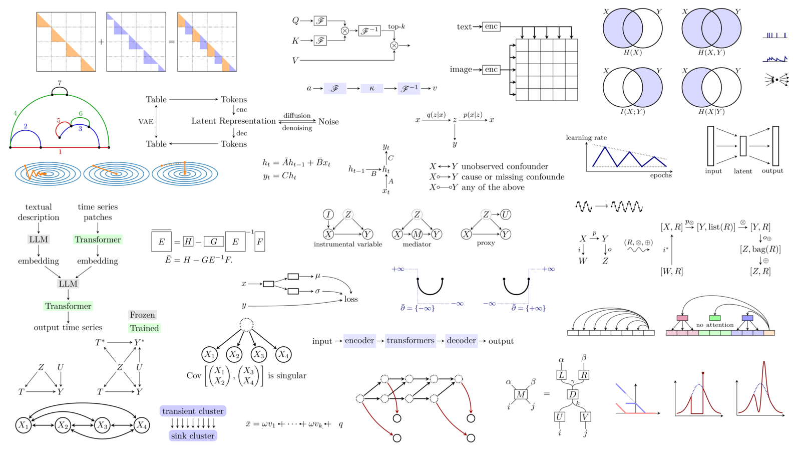
Causal discovery usually assumes that the data generation process defines a directed acyclic graph (DAG). This sounds like a reasonable assumption but, in some cases, we can end up with cycles. Here are a few examples.
Consider two variables, A and B evolving over time, the current value of each influencing the next value of the other. If we only observe the equilibrium state of that system, we have a cycle, A(∞)⇆B(∞).
In the same situation, A(t)→B(t+1) and B(t)→A(t+1), if we only observe aggregated data, a(t)=A(t)+A(t-1) and b(t)=B(t)+B(t-1), we have a circular relation between a and b. If the time scales are very different (e.g., seconds and months), we would have to add millions of unobserved variables: that is unreasonable.
On the three demons in causality in finance: time resolution, nonstationarity and latent factors
X. Dong et al. (2024)
https://arxiv.org/abs/2401.05414
Cyclic relations can also come from constraints: if A+B=1, then any intervention on A changes B, and conversely: each variable causes the other (in finance, this happens with portfolio weights).
Structural equation models (SEM) generalize structural causal models (SCM) by allowing cycles (and unobserved variables). If the model is linear, Gaussian, with known structure (the sparsity pattern, i.e., the directed graph, is known), it can be estimated by comparing the sample variance matrix of the observed variables with that of the model.
semopy: a Python package for structural equation modeling
G. Meschcheryakov and A.A. Igolkina (2019)
https://arxiv.org/abs/1905.09376

semopy 2: a structural equation modeling package with random effects in Python
G. Mosccheryakov et al. (2021)
https://arxiv.org/abs/2106.01140
To assess the quality of a causal discovery algorithm, we need to compare the predicted DAG with the ground-truth one.
The structural Hamming distance (SHD), the L¹ distance between the adjacency matrices, i.e., the number of edges to add or remove to recover the true graph, is an obvious choice, but it does not reflect the way the graph will be used -- to compute the causal impact of one variable on another.
Instead, the structural intervention distance (SID) counts how many times the parents of a node in the predicted graph are a valid adjustment set in the true graph.
Structural intervention distance (SID) for evaluating causal graphs
J. Peters and P. Bühlmann (2013)
https://arxiv.org/abs/1306.1043
This can be done with other valid adjustment sets, e.g., all previous nodes in a topological order, or the "optimal adjustment set" (optimal in terms of variance).
Adjustment identification distance: a gadjid for  causal structure learning
L. Henckel et al. (2024)
https://arxiv.org/abs/2402.08616

Graphical criteria for efficient total effect estimation via adjustment in causal linear models
L. Henkel et al. (2020)
https://arxiv.org/abs/1907.02435
Lesser-used distances include the number of conditional independencies entailed by one graph and not the other, or the number of causes (pairs of nodes with a causal path between them).
Investment decisions under almost complete causal ignorance
J. Simonian (2022)
Causal discovery algorithms are... disappointing. They tend to give very different results. To try to reduce the variability in their outputs, we could try to average them. But how can we average DAGs? Some majority vote, e.g., keeping the edges present in 50% (or some other threshold) of the graph gives a directed graph, but there is no guarantee that it will be acyclic.
This can be formulated as a combinatorial optimization problem: minimize the sum of the L¹ distances to the DAGs. The constraint that the graph be a DAG looks tricky, but it is actually easy to enforce: solve the problem without any constraint, check if there is a cycle, if there is one add the constraint that specific cycle, solve the problem again, and iterate, adding a new constraint each time you find a cycle. This is a sequence of mixed-integer linear programs (MIP).
Similarly, one can use a MaxSAT solver to combine background knowledge with the output of a causal discovery algorithm.
Introduction to the foundations of causal discovery
F. Eberhardt (2016)
https://link.springer.com/article/10.1007/s41060-016-0038-6
Assessing the quality of causal discovery algorithms is tricky: with real-world data, the ground truth causal graph is rarely known.
Instead, we can use simulated data, but it is very easy to introduce artefacts, which would not be present in real-world data, and help causal discovery -- for instance, variance tends to increase along a topological order.
Beware of the simulated DAG! Causal discovery benchmarks may be easy to game
A.G. Reisach et al. (2021)
https://arxiv.org/abs/2102.13647
The goal of causal inference is (once you have the causal graph) to estimate the causal effect of one variable ("treatment") T on another ("outcome") Y.
A straightforward approach is to control for the confounders (with more complex causal graphs, the notion of confounder should be replaced by "valid adjustment set"), i.e., to fit a model Y ~ T + X.
But controllong for confounders (aka backdoor adjustment, direct method) is not the only (or even the best) option. Inverse propensity weighting first fprecasts the treatment from the confounders, T ~ X, and then uses the predicted treatment probability ("propensity") as weights fo forecast the outcome.
"Doubly robust" methods combine controlling for confounders and inverse propensity weighting.
These are different estimators of the same quantity (the average treatment effect, or the conditional averate treatment effect) -- and there are many more: S-learner, T-learner, X-learner, double machine learning (DML), causal forests, etc.
Applied causal inference powered by ML and AI
V. Chernozhukov et al. (2024)
https://causalml-book.org/

Estimation and inference of heterogeneous treatment effects using random forests
S. Wager and S. Athey (2017)
https://arxiv.org/abs/1510.04342
For a concise and rigorous introduction to causal inference, check:
Causal Inference
N. Brady (2020)
https://www.bradyneal.com/causal-inference-course
For more details on the different causal inference procedures (controlling for confounders, inverse propensity weighting, doubly robust methods, etc.), check the following.
Causal inference in R workshop
https://www.youtube.com/watch?v=RyIyqV2LRvY
https://r-causal.github.io/causal_workshop_website/
Software for causal discovery include gcastle (which provides a unified API to the classical algorithms) and causal-learn (each algorithm has a different API, but it is easier to examine and change their inner components, e.g., the conditional independence tests for the PC algorithm).
https://github.com/huawei-noah/trustworthyAI/tree/master/gcastle
https://causal-learn.readthedocs.io/en/latest/
For causal inference, check dowhy.
https://github.com/py-why/dowhy
Machine learning and deep learning models are becoming larger, and it is increasingly difficult to understand what they are doing. We can attempt to address this issue in two ways: explainability and interpretability.
Explainability (XAI, explainable AI) takes a trained model, and tries to infer what it is doing, how it is using its inputs. For instance, partial dependency plots look at the average effect of changing one of the inputs while keeping the others constant; LIME approximates the model, in the neighbourhood of an observation, with a linear model; Shapley values decompose the output (separately for each sample) into a sum of contributions of the inputs. But XAI is only a rationalization of what the model is doing -- a plausible, convincing explanation, which can be completely wrong.
Interpretable machine learning
C. Molnar
https://christophm.github.io/interpretable-ml-book/
In contrast, interpretability seeks models that are interpretable by construction. Those models tend to be additive and/or sparse and/or monotonic and/or modular.
Designing inherently interpretable machine learning models
A. Sudjianto and A. Zhang (2021)
https://arxiv.org/abs/2111.01743
Let us list some of those models.
Interpretable and explainable machine learning: a methods-centric overview with concrete examples
R. Marcinkevičs and J.E. Vogt (2023)
https://wires.onlinelibrary.wiley.com/doi/full/10.1002/widm.1493
Linear models are interpretable, provided there is a small number of predictors: if there are many, a lasso or elasticnet penalty can help select a subset of them.
Statistical learning with sparsity
T. Hastie et al. (2015)
https://hastie.su.domains/StatLearnSparsity/
Interpretability can be improved further if you include some prior knowledge on the predictors: for instance, you often know whether they have a positive or negative effect on the target variable -- you can include those sign constraints in the regression. OLS is a quadratic optimization problem; you are just adding linear constraints: this is easily solved by a convex optimizer.
If the model is designed to be used by humans (this is often the case in medicine: "if this condition is satisfied, add 1 point; if that condition is satisfied, add 4 points; etc.; if the total to 10 or more, follow this procedure"), you can also ask for integer coefficients in the regression (this is a mixed integer optimization problem, which is still easy to solve -- scikit-learn's LinearRegression has a "positive" argument).
Supersparse linear integer models for interpretable classification
B. Ustun et al. (2014)
https://arxiv.org/abs/1306.6677

Supersparse linear integer models for optimized medical scoring systems
B. Ustun and C. Rudin
https://arxiv.org/abs/1502.04269
Some machine learning models readily accept monotonicity constraints, e.g., decision trees, or boosting (XGBoost, LightGBM, CatBoost all have an argument for that).
Decision trees are interpretable, but only if they are very shallow. Instead of learning balanced decision trees, whose branches quickly spread out, we can learn "1-dimensional" trees, or "rule lists": ask a question; if the answer is yes, return a forecast; if no, ask another question; iterate. "Falling rule lists" also add the condition that the forecast (say, the probability of a disease) decreases as you move along the list of questions.
An optimization approach to learning falling rule lists
C. Chen and C. Rudin (2018)
https://arxiv.org/abs/1710.02572
Linear regression does not account for... nonlinearities. Generalized additive models (GAM) are a straightforward generalization of linear models: each variable if first transformed, separately, in a nonlinear way; they are then combined linearly. It is possible to add monotonicity constraints, and it is also possible to combine GAMs with boosting: we do not end with with a single model, but a family of models (a "regularization path"), increasingly complex, in which the predictors enter one by one, initially in a linear fashion,
https://cran.r-project.org/web/packages/mboost/vignettes/mboost_tutorial.pdf
It is possible to add interactions, but care should be take to clearly separate the 1-variable effects from the interactions. GAMs can also be estimated with neural nets, or trees.
GAMI-Net: an explainable neural network based on generalized additive models with structured interactions
Z. Yang et al. (2020)
https://arxiv.org/abs/2003.07132

Interpretable machine learning based on functional Anova framework: algorithms and comparison
L. Hu et al. (2023)
https://arxiv.org/abs/2305.15670

Using model-based trees with boosting to fit low-order functional Anova models
L. Hu et al. (2022)
https://arxiv.org/abs/2207.06950
Neural nets are the archetypal example of non-interpretable models -- but this can be fixed, at least to some extent. For instance, we can constraint a neural network to be monotonic in its inputs.
The easiest way to do that is to use monotonic activation functions and positive weights. You should not (or not only) use ReLU for this: the network would be monotonic and convex in each of its inputs.
Constrained monotonic neural networks
D. Runje and S.M. Shankaranarayana (2022)
https://arxiv.org/abs/2205.11775
Alternatively, in particular if the model is more complex than a simple MLP, we can add a penalty on the gradient, to make it positive -- not the gradient of the loss wrt the parameters, which is used for training, but the gradient of the output wrt the input. The resulting model will be close to monotonic, but there is no guarantee.
How to incorporate monotonicity in deep networks while preserving flexibility?
A. Gupta et al. (2019)
https://arxiv.org/abs/1909.10662
If you need a guarantee that the model is monotonic (e.g., for legal reasons), monotonicity can be formulated as a satisfiability problem: this will give you a proof that the model is monotonic, regardless of how it was trained (or a proof that it is not).
Certified monotonic neural networks
X. Liu et al. (2020)
https://arxiv.org/abs/2011.10219
It is also possible to look for monotonicity counter-examples during training, and use them to make the model more monotonic.
Counterexample guided learning of monotonic neural networks
A. Sivaraman et al. (2020)
https://arxiv.org/abs/2006.08852
Making neural networks sparse (making them use only a small subset of their inputs) looks easy: just add an L¹ penalty to the coefficients of the first layer. In practice, however, it does not really work: none of the coefficients is exactly zero. To fix this, you can separate the L¹ penalty from the rest of the loss, and use proximal gradient.
Sparse-input neural networks for high-dimensional nonparametric regression and classification
J. Feng and N. Simon (2019)
https://arxiv.org/abs/1711.07592
Symbolic regression looks for a formula explaining the target variable from the predictors, using all the mathematical operators you provide. It may look appealing, but it is limited to situations with a small number of variables, and either a lot of data or very little noise -- it is good to find physical laws, but disappointing in many situations.
Interpretable machine learning with PySR and SymbolicRegression.jl
M. Cranmer (2023)
https://arxiv.org/abs/2305.01582
Additive index models (AIM) combine dimension reduction and GAM: they first project the input on a (learnt) low-dimensional space, and then fit a GAM on this space; the whole model is trained end-to-end.
Explainable neural networks based on additive index models
J. Vaughan et al. (2018)
https://arxiv.org/abs/1806.01933

Adaptive explainable neural networks (AxNNs)
J. Chen et al. (2020)
https://arxiv.org/abs/2004.02353
A variable coefficient model (VCM) is a locally linear model: a linear model in which the coefficients vary, but very slowly. To fit them, use a neural network, with a penalty to ensure the coefficients vary slowly.
Towards robust interpretability with self-explaining neural networks
D. Alvarez-Melis and T.S. Jaakola
https://arxiv.org/abs/1806.07538

Varying coefficient models
T. Hastie and R. Tibschirani (1993)
Some of those approaches can be combined, for instance, GAM and VCM.
Granger-causal attentive mixtures of experts: learning important features with neural nets
P. Schwab et al. (2019)
https://arxiv.org/abs/1802.02195
For a Python implementation of some of those models, check imodels (open source) or PiML (closed-source).
https://github.com/csinva/imodels
https://github.com/SelfExplainML/PiML-Toolbox
Under certain (reasonable) assumptions, the disagreement rate of the models in an ensemble (on unseen, unlabeled data) is a good estimator of the expected test accuracy.
On the joint interaction of models, data and features
Y. Jiang et al. (2024)
https://arxiv.org/abs/2306.04793

Assessing generalization via disagreement
Y. Jiang et al. (2021)
https://arxiv.org/abs/2106.13799
When you model a function with a deep learning model, one input gives one output: the model is always certain of its answers. Even if the output of the model is a probability distribution, it is rarely calibrated.
Surprisingly, it is possible to automatically calibrate those models -- any model. This is what conformal prediction does: it transforms any model into a model returning "confidence sets", guaranteed to contain the correct value α% of the time.
One idea (inductive conformal prediction, split conformal prediction) is to split the data in two, define a "non-conformity score" with the first split, and use the second split to decide how to use it to form confidence intervals. There are many possible choices for the non-conformity score; they can also be defined without splitting, with cross-validation or the Jackknife.
Another idea (transductive conformal prediction, full conformal prediction) is, given a new value of X, to refit the model with that new observation and all possible values of $y$.
Conformal prediction assumes exchangeability, i.e., that the order of the observations does not matter, which seems to exclude time series data, but there are a few work-arounds.
Distribution-free predictive uncertainty quantification: strength and limits of conformal prediction
(ICML 2024 tutorial)
https://icml.cc/virtual/2024/tutorial/35231

Introduction to conformal prediction with Python
C. Molnar (2023)
For Python implementations, check mapie, crepes, nixtla.
https://mapie.readthedocs.io/en/stable/
https://crepes.readthedocs.io/en/latest/
https://nixtlaverse.nixtla.io/statsforecast/docs/tutorials/conformalprediction.html
Recent, large models seem to require a huge amount of data. But it may be possible to achieve the same performance, with less data, provided we choose the training data wisely.
This is done, to some extent, when cleaning the data: deduplication, boilerplate removal (for text), identification to generated contents, etc.
Textbooks are all you need
S. Gunasekar et al. (2023)
https://arxiv.org/abs/2306.11644

The curse of recursion: training on generated data makes models forget
O. Shumailov et al. (2023)
https://arxiv.org/abs/2305.17493
But we can do more. For instance, during training, we can drop low-loss samples, or low-gradient samples, and train on the rest (you may need to adjust the gradients to reduce their bias).
InfoBatch: lossless training speed up by unbiased dynamic data pruning
Z. Qin et al. (2023)
https://arxiv.org/abs/2303.04947
You can also identify which samples are easy to learn and which are hard, by looking at the loss of a smaller, proxy models, and then decide to train on the easy ones (if you want to drastically reduce the size of the training set, focus on easy samples, if you can afford a larger training set, focus on the hard ones).
Towards a statistical theory of data selection under weak supervision
G. Kolossov et al.
https://arxiv.org/abs/2309.14563
For more details, and for applications to contrastive learning, check the following ICML tutorial.
Data-efficient machine learning
(ICML 2024 Tutorial)
https://icml.cc/virtual/2024/tutorial/35234
Data attribution looks at the opposite problem: once the model has been trained, which samples contributed the most?
Data attribution at scale
(ICML 2024 tutorial)
https://icml.cc/virtual/2024/tutorial/35228
The solution of the OLS problem is often written
ŷ = x' β
i.e., the forecast ŷ is a linear combination of the predictors y. But it can also be written
ŷ = x' β
  = [ x' (X' X )⁻¹ X' ] Y
  = w' Y
i.e., the forecast is a linear combination of the training set y's (the coefficients are data-specific: they depend on the new value x).
Those coefficients, known as "relevance" (of each training sample to the new observation) can be decomposed into a sum of 3 terms:
- The similarity (opposite of the Mahalanobis distance) between the new observation and each training sample;
- The informativeness of the new observation (distance to the average of the training data);
- The informativeness of each training sample.
Relevance-based forecasting uses those relevance weights, but only for the most relevant training samples.
Relevance
M. Czasonis et al.(2022)
https://globalmarkets.statestreet.com/research/service/public/v1/article/insights/pdf/v2/ecf31e52-64f3-49c7-84d7-19d6b70d5d0f/joim_relevance.pdf

Relevance-Based Prediction: A Transparent and Adaptive Alternative to Machine Learning
M. Czasonis et al.(2023)
https://globalmarkets.statestreet.com/research/service/public/v1/article/insights/pdf/v2/d0cdca66-3c68-4fd5-9608-f8953dc0ac78/jfds_relevance_based_prediction.pdf

A Transparent Alternative to Neural Networks with An Application to Predicting Volatility
M. Czasonis et al.(2024)
https://papers.ssrn.com/sol3/papers.cfm?abstract_id=4961917

The Virtue of Transparency: How to Maximize the Utility of Data without Overfitting
M. Czasonis et al.(2024)
https://papers.ssrn.com/sol3/papers.cfm?abstract_id=4903395

Portfolio construction when regimes are ambiguous
M. Kritzman et al. (2023)
https://globalmarkets.statestreet.com/research/service/public/v1/article/insights/pdf/v2/61df8160-4810-4cbe-8827-e6dc83a43dc8/jpm_portfolio_construction_when_regimes_are_ambiguous.pdf
We are familiar with supervised learning: we are given X (e.g., the features of a house: area, number of rooms, number of floors, presence of a pool, etc.) and y (the price of the house), for many examples, and we are asked to find a mapping from X to y.
In contrast, reinforcement learning focuses on decision making: we are given a "state" s (e.g., the location of the pieces on a chessboard) and we are asked fo find the best "action" a (the best move). To help us make that decision, we are given occasional "rewards" r (in the chess example, we only receive the reward at the end of the game, +1 or -1, depending on who wins).
The data used by supervised learning and reinforcement learning is very different. In supervised learning, we are give, a table with X and y columns; in reinforcement learning, we are given a table with 4 columns: current state s, action chosen a, reward r received immediately after that action, and next state s'.
The task is also very different. In supervised learning, we want to find a mapping from X to y. In reinforcement learning, there is also a mapping from state-action pairs, to reward and next state
s, a ↦ r, s'
but the goal is not to find that mapping, but to find the best action – a mapping ("policy") from state to action
π: s ↦ a
That task is fraught with difficulties.
- Contrary to supervised learning, we are never told what the best action is: the reward only tells us how good it is, not if it could have been better, or how to improve it -- the model will have to figure that out by itself.
- The rewards are delayed: we do not know immediately how good the action was: we may have to wait. Consequently, when we receive a reward, we do not know which action (or actions) contributed to it: some past actions could have been bad, some could have been good, but we do not know which ones. There could also be interactions between them: actions that would have been bad in isolation, but proved beneficial in combination with others.
- The state is constantly changing: an action is not good or bad in itself -- it could be good in one state and bad in another (e.g., in chess, losing a piece can be good if followed by other actions -- a gambit).
The multi-arm bandit (MAB) problem is a special case of reinforcement learning, in which there is no state: for eacg time step, we must choose an action ("arm") a∈⟦1,n⟧; we then receive a reward r ~ pₐ from some (unknown) distribution pₐ. We want a way of choosing the action (a "policy") to maximize the sum of the discounted rewards.
Here are a few policies.
ε-greedy keeps track of the average reward from each arm, pick the best one with probability 1-ε ("exploitation") and picks a random arm with probability ε ("exploration").
Thompson sampling assumes the data is Gaussian and keeps track of the (Bayesian) posterior distributions of the mean reward of each arm: to choose an arm, it samples a (random) reward from each of those posterior distributions, and picks the arm with the largest (sampled) reward.
UCB keeps track of a confidence interval for the mean of each arm, and picks that with the largest upper confidence bound.
Contextual bandits add state (but, contrary to reinforcement learning, there are no state transitions). The previous algorithms are straighforward to generalize: fit a model to predict the rewards of each arm from the context (the predictors, the state), e.g., with a linear regression (or some other machine learning model) and:
Pick the arm with the best forecast with probability 1-ε, and a random arm with probability ε (ε-greedy);
Use a Bayesian model to forecast the rewards, sample from the posterior expected reward, and pick the arm with the largest sampled reward (LinTS, Thompson sampling);
Use frequentist models, compute a confidence interval on their forecasts, and pick the arm with the largest upper confidence bound (LinUCB).
A contextual bandit approach to personalized news article recommendation
L. Li et al. (2010)
https://arxiv.org/abs/1003.0146

Thompson sampling for contextual bandits with linear payoffs
S. Agrawal and N. Goyal (2013)
https://arxiv.org/abs/1209.3352

Value-difference based exploration: adaptive control between epsilon-greedy and softmax
M. Tokic and G. Palm (2011)
http://www.tokic.com/www/tokicm/publikationen/papers/KI2011.pdf

Algorithms for the multi-armed bandit problem
V. Kuleshov and D. Precup (2009)
https://arxiv.org/abs/1402.6028
Traditional reinforcement learning maximizes the sum of discounted future rewards -- but we may want to maximize some other function of the rewards, e.g., the maximum, or some quantile (instead of the sum).
It is possible to adjust RL inforcement learning algorithms to arbitrary objective functions, e.g., by formulating the objective as an expectation (as with CVaR -- risk-seeking RL) or, as a last resort, by using f(r(≤t))-f(r(<t)) as rewards -- but you may need to augment the state space to ensure the decision process is still Markov.
Tackling decision processes with non-cummulative objectives using reinforcement learning
M. Nägele et al.
https://arxiv.org/abs/2405.13609
Large language models are traditionally trained in 2 steps: they are first trained to complete text, and then fine-tuned to work as an "assistant", answering queries, as helpfully as possible. That second step, "reinforcement learning with human feedback" (RLHF), uses reinforcement learning (RL): the model receives a reward, higher if the answer is more helpful. It would be impractical to ask humans to give those rewards directly: instead, there is an intermediate step (that makes 3 steps), in which we learn the reward function, from a few (human-annotated) examples; that reward function is then used for RL.
Learning the reward function is easy, but RL is hard. It turns out that those two steps can be fused: they then become a simple optimization problem (DPO).
Direct preference optimization: your language model is secretly a reward model
R. Rafailov et al. (2023)
https://arxiv.org/abs/2305.18290
Transformers were popularized for their applications to text, but they are not specifically targetted at sequence data -- on the contrary, they are permutation-invariant, i.e., the order of the tokens is ignored, unless it is provided separately, with a positional encoding.
Transformers can therefore also be applied to images, by using patches as tokens, and by replacing the 1-dimensional positional encoding with a 2-dimensional one (vision transformer, ViT). Surprisingly, the attention maps are not as informative as with text: tokens in low-information regions (e.g., the sky) appear important. It turns out that, since they were not useful to the model, the model decided to use them for internal computations. It is possible to recover the interpretability of the attention map by providing additional tokens ("registers") for the model to use for its internal computations.
Vision transformers need registers
T. Darcet et al.
https://arxiv.org/abs/2309.16588
Some applications of large language models require a modification of the sampling probabilities, for instance, for infilling q(B|A,C) ∝ p(ABC), or to add constraints q(A) ∝ p(A) c(A) (not on the next token, but on the next sequence of tokens). This can be done with GFlowNets, a diversity-seeking reinforcement learning algorithm.
Amortizing intractable inference in large language models
E.J. Hu et al. (2024)
https://openreview.net/forum?id=Ouj6p4ca60
The bag of tricks to train or use LLM models gets longer and longer. Here is a (far from exhaustive) random list.
To generate instruction-answer pairs for RLHF, use an LLM: start with the answers (good quality web pages) and ask an LLM to produce instructions that would lead to those answers.
Self-alignment with instruction back-translation
X. Li et al.
https://arxiv.org/abs/2308.06259
LLMs can be used to compress text: just ask them for a short prompt that will generate the desired text -- the result may not be human readable, but another model should be able to uncompress it.
Semantic compression with large language models
H. Gilbert et al. (2024)
https://arxiv.org/abs/2304.12512
One can also compress images in the same way.
If you do not know if you need RAG (retrieval-augmented generation) for a given query, you can just ask the LLM if it needs it.
Self-RAG: learning to retrieve, generate, and critique through self-reflection
A. Asai et al. (2023)
https://arxiv.org/abs/2310.11511
Instead of storing information in a vector store and querying it with RAG, one could store data in smaller LLMs -- ask each of those small LLMs to generate a document for the desired query, and proceed as if their answers came from a vector store.
Knowledge card: filling LLM's knowledge gaps with plugin specialized language models
S. Feng et al. (2024)
https://arxiv.org/abs/2305.09955
It is possible to recover most of a text from its embedding, by lerning an error-correcting model and applying it a few times.
Text embeddings reveal (almost) as much as text
J.X. Morris et al. (2023)
https://arxiv.org/abs/2310.06816
The LLMs we currently use are "foundational models" for text: they can be repurposed to any text-related task. There are efforts to build foundational models for other modalities: in particular for images, for tabular data, or for time series.
The current candidates for a "time series foundational model" (the examples below are not an exhaustive list) are still unconvincing: simpler approaches (ARIMA, N-BEATS, etc.) still perform better.
MOMENT: A family of open time-series foundation models
M. Goswami et al.
https://arxiv.org/abs/2402.03885

Lag-Llama: towards foundation models for probabilistic time series forecasting
K. Rasul et al.
https://arxiv.org/abs/2310.08278

A decoder-only foundation model for time series forecasting
A. Das et al.
https://arxiv.org/abs/2310.10688
Instead, one could try to re-purpose LLMs, from text to time series: freeze the transformers (the "intelligence") of the model, and only retrain the encoder (patch embedding) and decoder, for time series tasks
One Fits All: power general time series analysis by pretrained LM
T. Zhou et al.
https://arxiv.org/abs/2302.11939
Transformers can be used with time series, perhaps with a few modifications, such as using patches
A time series is worth 64 words: long-term forecasting with transformers
Y. Nie et al. (2022)
https://arxiv.org/abs/2211.14730
or replacing the products with convolution products,
Autoformer: decomposition transformers with autocorrelation for long-term series forecasting
H. Wu et al. (2021)
https://arxiv.org/abs/2106.13008
or operating in the frequency domain.
FEDFormer: frequency enhanced decomposed transformer for long-term series forecasting
T. Zhou et al. (2022)
https://arxiv.org/abs/2201.12740
Considering that foundational LLMs are a general form of intelligence, we can re-purpose them for time series: remove the first and last layers, which are text-specific, and replace them with time-series ones, and only train those, keeping the bulk of the network frozen. For the input, we can add both the numeric values of the time series (patches) and a textual description, if available.
Time-LLM: time series forecasting by reprogramming large language models
M. Jin et al.
https://arxiv.org/abs/2310.01728
Recurrent neural networks (RNN) are a very natural way of processing sequence data, but they have a short memory -- generalizations such as GRU or LSTM improve the situation, but not enough: they have been superseded by the transformer.
Unfortunately, the complexity of the transformer is quadratic in the context size. State space models may be able to revive RNNs and make them competitive with transformers.
A (continuous) state space model is of the form
ẋ = Ax + Bu
y = Cx + Du
where x is latent (hidden). It can be discretized into
xₖ = Ā xₖ₋₁ + ̄B uₖ
yₖ = ̄C xₖ
and solved with a convolution
y = ̄K * u.
Small technical details (FFT, diagonal-plus-low-rank parametrizations, gating, etc.) make it efficient and competitive with transformers. There is now a large number of such models: S4, Mamba, Hyena, etc.
Mamba: linear time sequence modeling with selective state spaces
A. Gu and T. Dao (2023)
https://arxiv.org/abs/2312.00752
Topological data analysis (TDA) looks for "holes" in data: for instance, a circle is a 1-dimensional hole. This can be used to detect periodic patterns in time series.
Topological time series analysis
J.A. Perea (2018)
https://arxiv.org/abs/1812.05143

Sliding windows and persistence: an application of topological methods to signal analysis
J.A. Perea and J. Harer (2013)
https://arxiv.org/abs/1307.6188
To detect a "changepoint" in a time series, look at the performance of a classification model predicting if t>t₀ from xₜ.
Random forests for change point detection
M. Londschien et al. (2023)
https://arxiv.org/abs/2205.04997
If there are potentially several change-points, use dynamic programming.
A kernel multiple change-point algorithm via model selection
S. Arlot et al. (2012)
https://arxiv.org/abs/1202.3878
When trying to minimize a function ℓ with gradient-based algorithms, its symmetries can help: if ℓ(g·x) = ℓ(x) for all x, we can replace the current solution candidate x with g·x; and we can choose g to make the gradient steeper -- this speeds up convergence, and may also improve generalization.
Improving convergence and generalization using parameter symmetries
B. Zhao et al. (2023)
https://arxiv.org/abs/2305.13404

Symmetry teleportation for accelerated optimization
B. Zhao et al. (2022)
https://arxiv.org/abs/2205.10637

Symmetries, flat minima, and the conserved quantities of gradient flow
B. Zhao et al. (2022)
https://arxiv.org/abs/2210.17216
To minimize a function f, we can consider a ball, moving on the graph of f, subject to both friction γ and acceleration: ẍ+γẋ+∇f(x)=0.
Stochastic heavy ball
S. Gadat et al. (2016)
https://arxiv.org/abs/1609.04228
We are familiar with "disciplined convex programming": a set of rules ensuring that an optimization problem is convex and amenable to convex solvers. This is what you are doing if you are using cvxpy.
This can be generalized to the search for saddle points.
Disciplined saddle programming
P. Schiele et al. (2023)
https://openreview.net/forum?id=KhMLfEIoUm
https://github.com/cvxgrp/dsp
Alpha mining, searching for simple models with good predictive powers, is often done with symbolic regression and genetic algorithms. Instead, one can use reinforcement learning to explore the space of formulas, maximizing, not the expected cummulated reward, but some quantile of it ("risk-seeking" reinforcement learning).
RiskMiner: discovering formulaic alphas via risk-seeking Monte Carlo tree search
T. Ren et al.
https://arxiv.org/abs/2402.07080
The stylized facts of financial time series are usually listed as fat fails, volatility clustering and, sometimes, leverage. There are actually more.
Modeling financial time series with generative adversarial networks
S. Takahashi et al. (2019)
Those stylized facts could be used to generate synthetic data, but the results are still unconvincing: synthetic financial data does not look or behave like real data.
Synthetic data applications in finance
V.K. Potluru et al. (2024)
https://arxiv.org/abs/2401.00081

Neural factors: a novel factor learning approach to generative modeling of equities
A. Gopal (2024)
https://arxiv.org/abs/2408.01499
In the long list of performance and risk measures, the entropic value at risk is becoming more popular.
Properties of the entropic risk measure EVaR in relation to selected distributions
Y. Mishura et al. (2024)
https://arxiv.org/abs/2403.01468
Risk may depend on the time scale (investing in stocks is risky in the short term, but less so in the long term): it can be decomposed into contributions of different time scales.
A new measure of risk using Fourier analysis
M. Grabinski and G. Klinkova (2024)
https://arxiv.org/abs/2408.10279
To build an investment strategy, one could forecast future stock returns and buy stocks with good forecasts. But not all those forecasts will be good: you may want to estimate how reliable those forecasts, and prefer stocks with good and reliable forecasts.
This can also be done at the portfolio level: look for a portfolio whose returns are (positive and) easy to forecast.
Canonical portfolios: optimal asset and signal combination
N. Firoozye et al. (2022)
https://arxiv.org/abs/2202.10817
Graph transformers (GAT) are not really graph neural networks: they are transformers whose positional encoding is given by the (eigenfunctions of the) Laplacian of the graph -- once that encoding is computed, the graph structure is discarded. But there are other options: you can use another graph kernel to compute the positional encoding; you can use a masked transformer (each node only attents to its k-hop neighbours); you can alternate transformer layers and message passing layers.
GraphiT: encoding graph structure in transformers
G. Mialon et al. (2021)
https://arxiv.org/abs/2106.05667

Recipe for a general, powerful, scalable graph transformer
L. Rampášek et al.
https://arxiv.org/abs/2205.12454
To make your graph neural net robust, divide the graph (the set of edges and/or features) into (non-overlapping) subgraphs, apply the model on each, and take the majority vote.
GNNCert: deterministic certification of graph neural networks against adversarial perturbations
Z. Xia et al. (2024)
https://openreview.net/forum?id=IGzaH538fz
For more on graph neural nets, and spectral methods (the graph Lapalcian and its eigenvalues), check this recent ICML tutorial.
Graph learning
(ICML 2024 Tutorial)
https://icml.cc/virtual/2024/tutorial/35233
Since neural networks are graphs, they can be processed by GNNs; applications include implicit neural representation (INR) classification; predicting the generalization performance of a network; improving the weights of a neural net (learning to optimize).
Graph neural networks for learning equivariant representations of neural networks
M. Kofinas et al.
https://arxiv.org/abs/2403.12143
Topological deep learning generalizes GNNs to higher-dimensional objects (simplicial complexes, hypergraphs, etc.).
Architectures of topological deep learning: a survey on topological neural networks
M. Papillon et al.
https://arxiv.org/abs/2304.10031
Diffusion models take samples from a distribution p₀ (the data, e.g., cat images), and adds noise to it, until we end up with samples from another distribution, p₁ (Gaussian). They then try to learn the reverse process: progressively denoising samples from p₁ until they look like samples from p₀.
They can do it using a stochastic process or a deterministic one.
Elucidating the design space of diffusion-based generative models
T. Karras et al.
https://arxiv.org/abs/2206.00364

Flow matching for generative modeling
Y. Lipman et al.
https://arxiv.org/abs/2210.02747
There are many choices available for those stochastic or deterministic processes.
Stochastic interpolants: a unifying framework for flows and diffusions
M.S. Albergo et al.
https://arxiv.org/abs/2303.08797
Adding more dimensions can help.
Poisson flow generative models
Y. Xu et al.
https://arxiv.org/abs/2209.11178

PFGM++: unlocking the potential of physics-inspired generative models
Y. Xu et al.
https://arxiv.org/abs/2302.04265
Diffusion models learn a denoising function (xₜ₊₁,t+1) ↦ xₜ; consistency models directly learn (xₜ,t) ↦ x₀.
Improved techniques for training consistency models
Y. Song and P. Dhariwal (2024)
https://arxiv.org/abs/2310.14189
Synthetic tabular data generation is still unconvincing.
Mixed-type tabular data synthesis with score-based diffusion in latent space
H. Zhang et al.
https://arxiv.org/abs/2310.09656
Research is still mostly focused on what to do with a single table -- but in real applications, we have several tables, sometimes even thousands of them...
Retrieve, merge, predict: augmenting tables with data lakes (experiment, analysis and benchmark paper)
R. Cappuzzo et al.
https://arxiv.org/abs/2402.06282
Optimal transport looks for a (deterministic) way of transforming one distribution p₀ into another p₁ (often, empirical distributions), in a deterministic way. The Schrödinger problem looks for stochastic processes instead.
A survey of the Schrödinger problem and some of its connections with optimal transport
C. Léonard (2014)
https://arxiv.org/abs/1308.0215
The optimal transport distance can be computed on mini-batches, but the result is biased.
Minibatch optimal transport distances; analysis and applications
K. Fatras et al.
https://arxiv.org/abs/2101.01792
Neural networks, when applied to time series or images, can be seen as working on the discretization of 1- or 2-dimensional functions.
We can replace the linear transformations used in neural nets with linear integral transforms: this allows the input to be provided on an arbitrary grid, and the output to be generated on an arbitrary grid.
Neural operator learning
(ICML 2024 tutorial)
https://arxiv.org/abs/2108.08481
ODEs are often used to model physical phenomena, but they may leave out some details: if the model is ẍ=f(x;θ), where f is known and θ is not (and has to be estimated from observational data), reality may be closer to ẍ=f(x;θ)+ε(x), where ε is a (small but) unknown function. Universal differential equations use neural nets to model ε.
Universal differential equations for scientific machine learning
C. Rackaukas et al. (2021)
https://arxiv.org/abs/2001.04385
Quantum computers do linear algebra in exponentially large vector spaces. This is what TDA needs (computing the rank of an exponentially large matrix): when quantum computers are available, they will provide more efficient TDA computations.
Topological data analysis on noisy quantum computers
I.Y. Akhalwaya et al.
https://arxiv.org/abs/2209.09371
While we wait for quantum computers, check giotto-tda, scikit-tda, gudhi, dionysus
giotto-tda: a topological data analysis toolkit for machine learning and data exploration
G. Tauzinb et al.
https://giotto-ai.github.io/gtda-docs/0.5.1/library.html
https://docs.scikit-tda.org/en/latest/
https://gudhi.inria.fr/python/latest/
https://github.com/mrzv/dionysus
In federated learning, the training data is not in a centralized location but is kept on "nodes" of a network, each node having access to only a subset of the data. A model can be trained with the "token" algorithm: each node updates the model parameters using its local gradient and sends the new values to one of its neighbours, at random. Instead of a random walk, we can use a self-repellent random walk: increase the probability of sending the token to nodes that have been visited less often.
Accelerating distributed stochastic optimization via self-repellent random walks
J. Hu et al.
https://arxiv.org/abs/2401.09665

Self-repellent random walks on general graphs: achieving minimal sampling variance via nonlinear Markov chains
V. Doshi et al. (2023)
https://arxiv.org/abs/2305.05097
Low-rank adaptation (LoRA) is a way of fine-tuning large language models with a small number of parameters: use W+BA' as weights, where W are the pre-trained weights (frozen) and A, B are smaller, trainable, rectangular matrices. One can also try other ways of modifying the weights matrix W, e.g., W⊙(BA').
Batched low-rank adaptation of foundation models
Y. Wen and S. Chaudhuri (2024)
https://arxiv.org/abs/2312.05677
There are many other variants or extensions of LoRA.
P-hacking is the search for small changes in an experiment (e.g., changes to hyperparameters) to make its results seem significant. But it can be sneakier: robust p-hacking looks for hyperparameters whose neighbourhood leads to significant results -- we could even ask for robustness to p-hacking detection tests.
Forking paths in financial economics
G. Coqueret (2023)
https://arxiv.org/abs/2401.08606
Decision trees, if they are too deep, will overfit the data. It is possible to have deep trees that overfit less, by introducing some shrinkage. Each node of a decision tree can output a forecast, which gets more precise and noisy (lower bias but higher variance) as we move deep into the tree. The final forecast (from the leaf), can be written as a telescopic sum, starting at the root, each term adding a correction to move one step down the branch.
yₙ = y₀ + ∑(yₖ-yₖ₋₁)
we can shrink those terms, e.g., with exponentially decreasing weights.
yₙ = y₀ + ∑γᵏ(yₖ-yₖ₋₁)

Hierarchical shrinkage: improving the accuracy and interpretability of tree-based methods
A. Agarwal et al. (2022)
https://arxiv.org/abs/2202.00858
https://github.com/csinva/imodels
If you want a (big) machine learning textbook from a Bayesian viewpoint, I recommend:
Probabilistic machine learning
K.P. Murphy (2022)
https://probml.github.io/pml-book/book1.html
(I have not read volume 2 yet...)
I have already mentioned some of the ICML tutorials:
Distribution-free predictive uncertainty quantification: strength and limits of conformal prediction
https://icml.cc/virtual/2024/tutorial/35231

Data-efficient machine learning
https://icml.cc/virtual/2024/tutorial/35234

Data attribution at scale
https://icml.cc/virtual/2024/tutorial/35228
The following may also be of interest.
Strategic machine learning is a generalization of adversarial machine learning: the users know the model (or parts of it) and change their features accordingly. (It is not always adversarial: for a recommendation system, the user will try to tweak the model to have better recommendations).
Strategic ML: learning with data that behaves
https://icml.cc/virtual/2024/tutorial/35230
Transformer-based models often end with a mixture of experts: the model can take several paths ("experts"), and decides which ones to take (with a "gating" mechanism).
Mixtures of experts in the era of LLMs
https://slideslive.com/39021919/mixtureofexperts-in-the-era-of-llms-a-new-odyssey?ref=folder-147931
In convex analysis, we would like to claim "every convex function has a minimum" -- but that is not true: convex functions can be unbounded. It is however possible to extend ℝⁿ in a way useful for complex analysis. (I am not convinced of the practical applications, but the tutorial was clear and interesting.)
Convex analysis at infinity: introduction to astral space
https://icml.cc/virtual/2024/tutorial/35232
https://arxiv.org/abs/2205.03260
posted at: 10:39 | path: /ML | permanent link to this entry
